
Automatic Differentiation for Matrices (Differentiable Programming)
Table of Contents
Introduction
In this notebook you will implement a class that supports automatic differentiation for matrices.
The idea is to implement individual operators like$ + $,$ * $ and the dot product and their derivatives. You can chain these operators together and construct expressions such as
C = A.dot(B + 3). These expressions apply the chain rule on the operators they're made up of to compute the derivatives.
Requirements
Prerequisites
- A notebook Automatic Differentiation for Scalars exists in which you implement a class that supports automatic differentiation for Scalar values rather than Matricies. You should complete the notebook on scalars first to get familiar with implementing an autodiff class and its operators. Then, move on to this notebook to tackle matricies.
Python Modules
import numpy as np
import numbers
import operator

from matplotlib import pyplot as plt
%matplotlib inline
Exercises
Derivative of the dot product
Assume a computational graph with a scalar output$ f $. However, the inner node can correspond to vector or matricies. In the computational graph, there is a vector variable node$ \vec y $.$ \vec y $ is computed in the forward pass by$ W \cdot \vec x $ (dot product).$ W $ is a matrix and$ \vec x $ is a vector.
The input$ \vec{x} $ has$ J $ elements, the output$ \vec {y} $ has$ I $ elements. So,$ \vec y(\vec{x}) $ maps a$ J $-dimensional vector$ \vec{x} $ to an$ I $-dimensional vector$ \vec{y} $.
$ \vec y : \mathbb{R}^J \to \mathbb{R}^I $
$ \vec y = W \cdot \vec x $
The scalar output$ f $ is an indirect function of$ \vec x $ via$ \vec y $:
$ f(\vec y) = f(\vec y(\vec x)) $
In the backward pass, we want to compute the gradient. The gradient w.r.t.$ \vec y $ is
$ \vec \nabla_y f = \vec \delta^{(y)} = \left(\frac{\partial f}{\partial y_1}, \frac{\partial f}{\partial y_2}, \dots, \frac{\partial f}{\partial y_I}\right)^T . $
The gradient (error responsibilities) w.r.t.$ \vec x $ is
$ \vec \nabla_x f = \vec \delta^{(x)} = \left(\frac{\partial f}{\partial x_1}, \frac{\partial f}{\partial x_2}, \dots, \frac{\partial f}{\partial x_J}\right)^T . $
Vectorized Chain Rule and Jacobian Matrix
The vectorized chain rule is: $ \frac{\partial f}{\partial \vec{x}} = \frac{\partial f}{\partial \vec{y}} \cdot \frac{\partial \vec{y}}{\partial \vec{x}}. $
What the meaning of$ \frac{\partial \vec{y}}{\partial \vec{x}} $?
$ \frac{\partial \vec{y}}{\partial \vec{x}} $ is a matrix (see below). To make this more clear, we use the following notation$ \left[ \frac{\partial \vec{y}}{\partial \vec{x}} \right] $.
In our case the relation between$ \vec x $ and$ \vec y $ is given by the matrix multiplication$ \vec y = W \cdot \vec x $.
As an example, the input has 3 elements$ x_1 $,$ x_2 $ and$ x_3 $ and the output has two elements$ y_1 $ and$ y_2 $:

We want to derive each output feature$ y_i $ with respect to$ \vec{x} $. So let's expand the features of$ \vec{y} $ into a vector. $ \frac{\partial \vec{y}}{\partial \vec{x}} = \begin{bmatrix} \frac{\partial y_1}{\partial \vec{x}}\\ \frac{\partial y_2}{\partial \vec{x}}\\ \end{bmatrix} $
Let's take it a step further - we want derive each output feature with respect to each input feature. So, let's expand the features of$ \vec{x} $ as columns.
$ \left[\frac{\partial \vec{y}}{\partial \vec{x}}\right] = \begin{bmatrix} \frac{\partial y_1}{\partial \vec{x}}\\ \frac{\partial y_2}{\partial \vec{x}}\\ \end{bmatrix} = \begin{bmatrix} \frac{\partial y_1}{\partial x_1} & \frac{\partial y_1}{\partial x_2} & \frac{\partial y_1}{\partial x_3}\\ \frac{\partial y_2}{\partial x_1} & \frac{\partial y_2}{\partial x_2} & \frac{\partial y_2}{\partial x_3}\\ \end{bmatrix} $
This gives us a matrix of all partial derivatives, which is also called the Jacobian matrix.
Let's get the actual values of the derivatives for the matrix multiplication. here, the output elements were computed by:
$ y_1 = w_{11} * x_1 + w_{12} * x_2 + w_{13} * x_3\\ y_2 = w_{21} * x_1 + w_{22} * x_2 + w_{23} * x_3 $
Now, let's focus on the single input element$ x_1 $. The graph below shows how$ x_1 $ contributes to the output. Note: In the full computational graph, there are more arrows pointing to$ y_1 $ and$ y_2 $ which are not shown in the graph.
To derive$ f $ with respect to$ x_1 $, we must sum over all paths to which$ x_1 $ contributes (multivariable chain rule). So:
\begin{equation} \delta_1^{(x)} = \frac{\partial f}{\partial x_1} = \frac{\partial f}{\partial y_1} \frac{\partial y_1}{\partial x_1} + \frac{\partial f}{\partial y_2} \frac{\partial y_2}{\partial x_1} \end{equation}
or in general:
\begin{equation} \delta_j^{(x)} = \sum_i \frac{\partial f}{\partial y_i} \frac{\partial y_i}{\partial x_j} \label{eq:delta_x} \tag{1} \end{equation}
Task:
Show that the gradient w.r.t$ \vec x $ is $ \vec \delta^{(x)} = W^T \vec \delta^{(y)}. $
Hint: Use equation$ \eqref{eq:delta_x} $.
Row vectors
In the previous exercise,$ \vec x $ was a column vector. If$ \vec a $ is a row vector instead, the order of$ \vec a $ and$ V $ is reversed in the dot product (forward pass).
$ \vec b : \mathbb{R}^J \to \mathbb{R}^I $
$ \vec b = \vec a \cdot V $ Note$ \vec b $ is also a row vector.
$ f(\vec b) = f(\vec b(\vec a)) $
Task
How do we calculate$ \vec \delta^{(a)} $ in vectorized form now?
Note:$ \vec \delta^{(a)} $ is now a row vector.
Matrix-Matrix product
We can generalize what we learnt about the matrix-vector product chain rule to a matrix-matrix product.
We have: $ W \cdot X = Y $ $ X $ and$ Y $ are now matricies. Both have$ K $-columns.
Note that the matrix-matrix dot product is equivalent to:
$ W \cdot X = \begin{pmatrix}W \vec x_1 & W \vec x_2 & \dots & W \vec x_K \end{pmatrix} = \begin{pmatrix} \vec y_1 & \vec y_2 & \dots & \vec y_K \end{pmatrix} = Y $ with
- the column vectors$ \vec x_k $ of$ X $ and
- the column vectors$ \vec y_k $ of$ Y $.
In other words, a column vector of$ Y $ is computed by the dot product of$ W $ with a column vector of$ X $:
$ \vec y_k = W \cdot \vec x_k $
From our result above, we know that the gradient vectors are connected by
$ \vec \delta_k^{(x)} = W^T \cdot \vec \delta_k^{(y)}. $
We store all values of the$ \vec \delta_k^{(x)} $ and$ \vec \delta_k^{(y)} $ in the matricies$ \hat \delta^{(x)} $ respectively$ \hat \delta^{(y)} $. The$ \vec \delta_k^{(x)} $ and$ \vec \delta_k^{(y)} $ are the column vectors of the matricies. Then the "backprop rule" for the dot-product$ Y=W\cdot X $ is:
$ \hat \delta^{(x)} = W^T \cdot \hat \delta^{(y)} $
Task
For the dot-product$ Y=W\cdot X $:
What is the "backprop rule" for$ \hat \delta_k^{(w)} $?
Autodiff class Node
Deep learning frameworks support automatic differentiation via backpropagation through the computational graph. To demonstrate how autodiff works we implement an autodiff python class Node.
The syntax of this class should be familiar to you from the exercise Automatic Differentiation for Scalars (see Requirements) - so we won't go as much into detail about it again.
Note: We have to add multiple path to the same variable as the multivariable chain rule tells us. In the implementation, we store the partial derivatives in a python dictionary. We need a helper function combine_dicts for taking the multivariate chain rule into account (see notebook Automatic Differentiation for Scalars ):
def combine_dicts(a, b, op=operator.add):
    x = (list(a.items()) + list(b.items()) +
        [(k, op(a[k], b[k])) for k in set(b) & set(a)])
    return {x[i][0]: x[i][1] for i in range(0, len(x))}
# Here you see how combine dicts work
a = {'a': 2, 'b':3, 'c':4}
b = {'a': 5, 'c':6, 'x':7}
combine_dicts(a, b)# and another example
A = {'a':-1.3, 'b':-4, 'c':3}
B = {'b':3, 'c':4, 'd':5}
combine_dicts(A,B)Node class
Below is a skeleton for the node class and a number of helper functions.
class Node(object):

    def __init__(self, value, name=None):
        value = Node._wrap_2d(value)
        self._set_variables(name, value)
        # only 2D-Arrays are supported at the moment
        assert len(self.shape)==2


    # Sets input variables and provides the grad function
    def _set_variables(self, name, value):
        self.value = value

        # add shape and dtype for Node
        self.shape = value.shape
        self.dtype = value.dtype

        # analog to notebook "Automatic Differentiation for Scalars":
        self.name = name
        if name:
            self.grad = lambda g : {name : g}
        else:
            self.grad = lambda g : {}
2D Helper
The value of each Node is a 2D numpy array. This consistency is important. All operators we're going to implement handle 2D numpy arrays. Node objects are initialized with a value and optionally a name.
Task: Implement the _wrap_2d helper function.
- If the argument
valueis a scalar, returnvalueas a 2D numpy array (shape (1,1)) - If
valueis a 1D (numpy) array, return it as a 2D column vector (shape (n,1))
# Ensure that the value is a 2D numpy array.
# Scalars and 1D values are wrapped as a 2D array.
def _wrap_2d(value):
    raise NotImplementedError()

# add to Node class
Node._wrap_2d = _wrap_2d
assert np.array_equal([[3]], Node(3).value)
assert np.array_equal([[3]], Node(np.array([3])).value)
assert np.array_equal([[3]], Node(np.array([[3]])).value)
assert Node(np.array([1,2,3])).shape == (3,1)Operators
Now we can start adding operators and their derivatives. The syntax should be familiar to you from the notebook Automatic Differentiation for Scalars.
The only things that have changed:
- The
valueof each node is a 2D array.
Note that the addition is only allowed for 2D arrays that have equal shape. We are going to handle broadcasting later.
def __add__(self, other):

    # if the the value of other is a number wrap it in a Node:
    if isinstance(other, numbers.Number):
        other = Node(np.array([[other]]))

    # forward pass
    ret = Node(self.value + other.value)

    # for backward pass
    def grad(g):
        # derivative root w.r.t self and other
        g_total_self = g
        g_total_other = g
        x = combine_dicts(self.grad(g_total_self), other.grad(g_total_other))
        return x
    ret.grad = grad
    return ret

Node.__add__ = __add__
To make this more clear, we use an example.
Assume we have an add-node in our computational graph:
$ C = A + B $ with the$ I\times J $-matricies$ A $, $ B $ and $ C $.
The scalar output of the graph is $ f = \sum_{ij} C_{ij} $
The gradient vector is defined by the vectorized version of$ C $, e.g., $ \vec c $ with elements$ c_k $ $ K $ is the number of elements). Each$ c_k $ correspond to a entry of the matrix$ C_{ij} $, so$ K=I*J $
$ \frac{\partial f}{\partial \vec c} = \begin{pmatrix} \frac{\partial f}{\partial c_1}\\ \vdots \\ \frac{\partial f}{\partial c_k}\\ \vdots \\ \frac{\partial f}{\partial c_K}\\ \end{pmatrix} $
However, that's not the way we implement it. In the implementation, we use a matrix for the gradient of$ f $ with respect to$ C $:
$ \frac{\partial f}{\partial C} = \begin{pmatrix} \frac{\partial f}{\partial C_{11}} & \dots & \frac{\partial f}{\partial C_{1j}} &\dots & \frac{\partial f}{\partial C_{1J}}\\ \vdots & \ddots & \vdots & \ddots & \vdots\\ \frac{\partial f}{\partial C_{i1}} & \dots & \frac{\partial f}{\partial C_{ij}} &\dots & \frac{\partial f}{\partial C_{iJ}}\\ \vdots & \ddots & \vdots & \ddots & \vdots \\ \frac{\partial f}{\partial C_{I1}} & \dots & \frac{\partial f}{\partial C_{Ij}} &\dots & \frac{\partial f}{\partial C_{IJ}}\\ \end{pmatrix} $
Task
What values have the entries of$ \frac{\partial f}{\partial C_{ij}} $.
Note: You need the result to implement the sum operator.
From the multivariate chain rule $ \frac{\partial f}{\partial b_{l}} = \sum_{k} \frac{\partial f}{\partial c_{k}}\frac{\partial c_{k}}{\partial b_{l}} $
follows for our matrix version: $ \frac{\partial f}{\partial B_{ij}} = \sum_{m,n}\frac{\partial f}{\partial C_{mn}}\frac{\partial C_{mn}}{\partial B_{ij}} $
For the matrix addition, we have $ \frac{\partial C_{mn}}{\partial B_{ij}} = \delta_{mi} \delta_{nj} $
So, we get $ \frac{\partial f}{\partial B_{ij}} = 1 $ for all$ i,j $-pairs.
This seems to by an overcomplicated derivation for a simple result. However, we need a similar derivation to show how broadcasting works.
If the argument is a number, we wrap it as a Node so both of the expressions node + 1 and node + Node(1) are equivalent and valid.
node = Node(np.arange(6).reshape((2,3)))
a = (node + 1).value
b = (node + Node(1)).value
assert np.array_equal(a, b)
The way we compute gradients is similar to how we handled scalars, see Automatic Differentiation for Scalars for a more detailed explanation.
We use the helper function
Node._set_grad(self, g_total_self, other, g_total_other) which
- handles broadcasting
- calls self.grad(g_total_self)
- calls other.grad(g_total_other)
This produces a dictionary of gradients for each branch leading up to C. The function combines these gradients and returns the combined dictionary.

Task: Implement the Sum-Operator
Here, should implement a _sum_all()-operator.
In the forward pass, _sum_all() should add up all elements of the input matrix.
The output is a matrix with shape$ (1,1) $.
So, we can use it to realize the f-node output of the example above.
We call the operation _sum_all() because there is no axis-argument.
Optionally (for experts): Implement a sum()-operator which supports an axis-argument.
def _sum_all(self):
    ret = None # Your work
    def grad(g):
        x = None # Your work
        return x
    ret.grad = grad
    return ret


Node.sum_all = _sum_all
Operators - Multiply
Assume we have an element-wise multiplication (*) node
in our computational graph:
$ C = A * B $ with the$ I\times J $-matricies$ A $, $ B $ and $ C $.
The scalar output of the graph is $ f = \sum_{ij} C_{ij} $
What is$ \frac{\partial f}{\partial B_{ij}} $?
Hint: Use the matrix version of the multivariate chain rule
$ \frac{\partial f}{\partial B_{ij}} = \sum_{m,n}\frac{\partial f}{\partial C_{mn}}\frac{\partial C_{mn}}{\partial B_{ij}} $
Task: Implement the (element-wise) multiplication operator.
def __mul__(self, other):
    raise NotImplementedError()

Node.__mul__ = __mul__
# implicit forward pass:
a = Node(np.array([[1,1,1], [2,2,2]]), "A")
b = Node(np.array([[10, 20, 30], [10, 20, 30]]), "B")
c = a * b
f = c.sum_all()
assert np.array_equal(c.value, np.array([[10, 20, 30], [20, 40, 60]]))
# backward pass:
grads = f.grad(1) # gradient of C w.r.t A and B
assert np.array_equal(grads['A'], np.array([[10, 20, 30], [10, 20, 30]]))
assert np.array_equal(grads['B'], np.array([[1, 1, 1], [2, 2, 2]]))Broadcasting
This was our first trial to implement + and *.
However, what happens if we want to use broadcasting, e.g.:
a = Node(np.array([[1,1], [2,2]]), "a")
b = Node(np.array([[10, 20]]), "b")
c = a * b
f = c.sum()
To make this more clear, we use our modified example.
Assume we have an element-wise multiplication-node in our computational graph (which supports broadcasting):
$ C = A * B $ with the$ I\times J $-matricies$ A $ and$ C $.$ B $ is now a$ 1 \times J $-matrix.
The scalar output of the graph is $ f = \sum_{ij} C_{ij} $
Note that broadcasting tells us how to compute an element of$ C $:
$ C_{mn} = A_{mn} * B_{1n} $
We can use the multivariable chain rule to show how braodcasting must be taken into account for backprop:
For the gradient w.r.t.$ B $: $ \begin{align} \frac{\partial f}{\partial B_{1j}} &= \sum_{m,n}\frac{\partial f}{\partial C_{mn}}\frac{\partial C_{mn}}{\partial B_{1j}} \\ &= \sum_{m,n}1 * \frac{\partial\left( A_{mn} * B_{1n} \right)}{\partial B_{1j}} \\ &= \sum_{m} \frac{\partial\left( A_{mj} * B_{1j} \right)}{\partial B_{1j}} \\ &= \sum_{m} A_{mj}\\ \end{align} $
and the gradient w.r.t.$ A $:
$ \begin{align} \frac{\partial f}{\partial A_{ij}} &= \sum_{m,n}\frac{\partial f}{\partial C_{mn}}\frac{\partial C_{mn}}{\partial A_{ij}} \\ &= \sum_{m,n}1 * \frac{\partial\left( A_{mn} * B_{1n} \right)}{\partial A_{ij}} \\ &= \sum_{m} \frac{\partial\left( A_{mj} * B_{1j} \right)}{\partial A_{ij}} \\ &= B_{1j} \end{align} $
Task
Maybe, this was a litle bit to abstract. To make it more clear work through the example in pen & paper exercise:
$ A =\begin{pmatrix} 1 & 1 \\ 3 & 4 \end{pmatrix} $
and$ C = A*B $ using broadcasting. The output node is$ f = \sum_{ij} C_{ij} $.
- What is the
shapeof$ C $? - What is the
shapeof the gradient$ \frac{\partial f}{\partial B} $? - Compute by hand the gradient of$ f $ w.r.t. (with respect to)$ A $, i.e.$ \frac{\partial f}{\partial A} $.
- Compute by hand the gradient of$ f $ w.r.t. (with respect to)$ B $, i.e.$ \frac{\partial f}{\partial B} $. Which rule have we take into account for computing the gradient w.r.t.$ B $?
Hint: Think about "How are the four elements of$ C $ computed by the two elements of$ B $. How many paths (in backward direction) are going to the elements of$ B $?" You can also use a computational graph with nodes for all elements of$ A SINGLE``SINGLE B $ and$ C $ (as in the exercises above).
Implementation of broadcasting
So, broadcasting make things slightly more complicated.
We have to take the multivariable chain rule into account.
So, we must sum over all pathes in the implementation of
_broadcast_g_helper for our Node-class:
def _broadcast_g_helper(o, o_):
    # Take the multivariable chain rule into account:
    if o_.shape[0] > o.shape[0]:
        o_ = o_.sum(axis=0).reshape(1,-1)
    if o_.shape[1] > o.shape[1]:
        o_ = o_.sum(axis=1).reshape(-1,1)
    return o_

Node._broadcast_g_helper = _broadcast_g_helper
For all binary operators, we have to call the broadcast helper
for both branches, call the grad function of each input and have to combine the dicts. So, we write a convenience function _set_grad for our Node-class:
def _set_grad(self_, g_total_self, other, g_total_other):
        g_total_self = Node._broadcast_g_helper(self_, g_total_self)
        g_total_other = Node._broadcast_g_helper(other, g_total_other)
        x = combine_dicts(self_.grad(g_total_self), other.grad(g_total_other))
        return x

Node._set_grad = _set_grad
Our new implementation of __add__ is nearly the same.
Only one line changes:
def __add__(self, other):

    # if the the value of other is a number wrap it in a Node:
    if isinstance(other, numbers.Number):
        other = Node(np.array([[other]]))

    # forward pass
    ret = Node(self.value + other.value)

    # for backward pass
    def grad(g):
        # derivative root w.r.t self and other
        g_total_self = g
        g_total_other = g
        # this is the only change we have to do:
        # this line is replaced by
        # x = combine_dicts(self.grad(g_total_self), other.grad(g_total_other))
        # this
        x = Node._set_grad(self, g_total_self, other, g_total_other)

        return x

    ret.grad = grad
    return ret

Node.__add__ = __add__
Task
Implement the new version of __mul__.
You just have to copy g_total_self and g_total_other from your __mul__-implementation above.
def __mul__(self, other):
    if isinstance(other, numbers.Number) or isinstance(other, np.ndarray):
        other = Node(other)
    ret = Node(self.value * other.value)
    def grad(g):
        g_total_self = None #Your task
        g_total_other = None # Your task
        x = Node._set_grad(self, g_total_self, other, g_total_other)
        return x
    ret.grad = grad
    return ret

Node.__mul__ = __mul__
# This is the example of the pen & paper exercise:
A = Node(np.array([[1,2], [3,4]]), "A")
B = Node(np.array([[10, 20]]), "B")
C = A * B
f = C.sum_all()
grads = f.grad(1)
#print(grads) # comment this out and compare it with your pen & paper result.# Test for the element-wise multiplication
# implicit forward pass:
a = Node(np.array([[1,1,1], [2,2,2]]), "A")
b = Node(np.array([[10, 20, 30]]), "B")
c = a * b
f = c.sum_all()
assert np.array_equal(c.value, np.array([[10, 20, 30], [20, 40, 60]]))
# backward pass:
grads = f.grad(1) # gradient of C w.r.t A and B
assert np.array_equal(c.value, np.array([[10, 20, 30], [20, 40, 60]]))
assert np.array_equal(grads['A'], np.array([[10, 20, 30],[10, 20, 30]]))
assert np.array_equal(grads['B'], np.array([[3,3,3]]))Operators - Dot product
Task: Implement the dot product. The exercise derivative of the dot product mentions how to differentiate the dot product operator.
def dot(self, other):
    raise NotImplementedError()

Node.dot = dot
Verify your implementation.
a = Node(np.array([[1,2,3],
       [4,5,6]]), "a")
b = Node(np.array([[10,10],
        [20,20],
        [30,30]]), "b")
c = dot(a,b)
assert np.array_equal(c.value, np.array([[140, 140], [320, 320]]))
assert np.array_equal(c.grad(1)['a'], np.array([[10, 20, 30], [10, 20, 30]]))
assert np.array_equal(c.grad(1)['b'], np.array([[1, 4], [2, 5], [3, 6]]))
Operators - Square
Task: Implement the square operator.
def square(self):
    raise NotImplementedError()

Node.square = square
# Test for the square-operator
a = Node(np.array([[1,2,3], [4,5,6]]), "a")
b = a.square()
f = b.sum_all()
assert np.array_equal(b.value, np.array([[ 1, 4, 9], [16, 25, 36]]))
assert np.array_equal(b.grad(1)['a'], np.array([[ 2, 4, 6],[ 8, 10, 12]]))Additional operators
We extend the Node class with some more operators (which are already fully implemented).
Task
What are the meanings of the python magic functions? Look the meaning up in https://docs.python.org/3/library/operator.html
def __radd__(self, other):
    return Node(other) + self

def __sub__(self, other):
    if isinstance(other, numbers.Number):
        other = Node(other)
    ret = self + (other * -1.)
    return ret

def __rsub__(self, other):
    if isinstance(other, numbers.Number):
        other = Node(other)
        return other - self
    raise NotImplementedError()

def __rmul__(self, other):
    if isinstance(other, numbers.Number):
        return Node(other) * self
    raise NotImplementedError()


def __truediv__(self, other):
    if isinstance(other, numbers.Number):
        other = Node(np.array([[other]]))
    ret = Node(self.value / other.value)
    def grad(g):
        g_total_self = g / other.value
        g_total_other = -1 * self.value * g / (other.value**2)
        x = Node._set_grad(self, g_total_self, other, g_total_other)
        return x
    ret.grad = grad
    return ret

def __rtruediv__(self, other):
    if isinstance(other, numbers.Number):
        other = Node(other)
        return other/self
    raise NotImplementedError()

def __neg__(self):
    return self * -1.

def _sum_(self, axis=None):
    if axis is None:
        return self.sum_all()
    assert axis in (0,1)
    return self._sum(axis)

def _sum(self, axis):
    ret = self.value.sum(axis=axis)
    if axis==0:
        ret = ret.reshape(1, -1)
    else:
        ret = ret.reshape(-1, 1)
    ret = Node(ret)
    def grad(g):
        x = self.grad(np.ones_like(self.value) * g)
        return x
    ret.grad = grad
    return ret


Node.__radd__ = __radd__
Node.__sub__ = __sub__
Node.__rsub__ = __rsub__
Node.__rmul__ = __rmul__
Node.__truediv__ = __truediv__
Node.__rtruediv__ = __rtruediv__
Node.__neg__ = __neg__
Node._sum = _sum
Node.sum = _sum_
Node class for Softmax Regression
Here, we want to use the node class for Softmax regression.
Setup for an example data set:
# class 1
# covariance matrix and mean
cov1 = np.array([[4,-1],[-1,4]])
mean1 = np.array([4,4])
# number of data points
m1 = 100

# class 2
# covariance matrix
cov2 = np.array([[3,1.5],[1.5,3]])
mean2 = np.array([-2.,5])
# number of data points
m2 = 100

# class 3
# covariance matrix
cov3 = np.array([[3,1],[1,3]])
mean3 = np.array([0,-1])
# number of data points
m3 = 100

# generate m gaussian distributed data points with
# mean and cov.
r1 = np.random.multivariate_normal(mean1, cov1, m1)
r2 = np.random.multivariate_normal(mean2, cov2, m2)
r3 = np.random.multivariate_normal(mean3, cov3, m3)


X = np.concatenate((r1,r2,r3))
y = np.ones(X.shape[0], dtype=np.int32) * 2
y[:len(r1),] = 0
y[len(r1):len(r1)+len(r2)] = 1plt.figure(figsize=(8,8))
x1_min= x2_min= -6
x1_max= x2_max= 10
plt.xlim(x1_min, x1_max)
plt.ylim(x2_min, x2_max)
plt.scatter(r1[...,0], r1[...,1], c='r', marker='x', label="class 0")
plt.scatter(r2[...,0], r2[...,1], c='b', marker='o', label="class 1")
plt.scatter(r3[...,0], r3[...,1], c='g', marker='*', label="class 2")
plt.xlabel("$x_1$")
plt.ylabel("$x_2$")
plt.legend()
plt.show()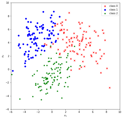
# Add one column for the bias trick
def add_x0(X):
    one_vec = np.ones((X.shape[0],1))
    return np.concatenate((one_vec, X), axis=1)

X_train = add_x0(X)
# convert y to one-hot
nb_training_data = y.shape[0]
nb_classes = int(y.max()+1)
y_oh = np.zeros((nb_training_data, nb_classes))
y_oh[range(nb_training_data), y] = 1.THETA = "theta"
def Softmax_regression_model(theta_, x, y_oh=None):
# y_oh: one-hot labels
X = Node(x) # no name -> no grad
W = Node(theta_, name=THETA) # name -> grad
f = X.dot(W)
h = f.softmax()
if y_oh is not None: # cost function
t = Node(y_oh)
assert t.shape == h.shape
loss = - t * h.log()
cost = loss.sum()
return h, cost
return hOnce we've computed the loss, we call its grad function loss.grad(np.ones_like(loss.value)) and get the gradients for all parameters in the forward pass. We apply these gradients in gradient descent.
def gradient_descent(x, y, epochs, theta, alpha=0.001):

    #out, cost = Softmax_regression_model(theta, x, y)

    for i in range(epochs):

        out, cost = Softmax_regression_model(theta, x, y)
        if i%200==0:
            print (i, cost.value)

        #backprop
        grad = cost.grad(1.)
        for g in grad:
            assert g==THETA # we only have only one parameter (matrix)
            gradient = grad[g]
            assert theta.shape == gradient.shape
            theta -= alpha * gradient
    return theta
Task: Operators for Softmax Regression
Implement exp, log and softmax for the Node-class.
Write tests to check your implementation.
Note: For the tests, you should compute by pen and paper numeric values for small computational graphs using the operators. Check the numeric values in the tests.
#
def exp(self):
    raise NotImplementedError()

def log(self):
    raise NotImplementedError()

def softmax(self):
    raise NotImplementedError()

Node.softmax = softmax
Node.exp = exp
Node.log = log
Now, we'll use gradient descent to map points in (x,y) coordinates to a target class 0 or 1. In the plot below, the green line marks all points (x,y) where the output of the model is 0.5. It serves as a decision boundary for the model.
theta_fit = gradient_descent(X_train, y_oh, 1000,
                             np.zeros((3, nb_classes)), alpha=0.002)

# use a closure to store theta_fit for a prediction model
model = lambda x: Softmax_regression_model(theta_fit, x, y_oh=None)
0 [[329.5836866]]
200 [[50.75304675]]
400 [[49.17330126]]
600 [[48.67656768]]
800 [[48.44235252]]
def plot_prediction(model, X, targets=y):
    fig = plt.figure(figsize=(8,8))

    x1_min= x2_min= -6
    x1_max= x2_max= 10
    plt.xlim(x1_min, x1_max)
    plt.ylim(x2_min, x2_max)

    delta = 0.1
    a = np.arange(x1_min, x1_max+delta, delta)
    b = np.arange(x2_min, x2_max+delta, delta)
    A, B = np.meshgrid(a, b)

    x_ = np.dstack((A, B)).reshape(-1, 2)
    out = model(add_x0(x_)).value

    ns = list()
    ns.append(3)
    ns.extend(A.shape)

    out = out.T.reshape(ns)

    # TODO: fix colors
    plt.pcolor(A, B, out[0], cmap="copper", alpha=0.2)
    plt.pcolor(A, B, out[1], cmap='Reds', alpha=0.2)
    plt.pcolor(A, B, out[2], cmap='Blues', alpha=0.2)
    #out.shape
    # lets visualize the data:
    # TODO: fix colors for data points
    plt.scatter(X[:, 1], X[:, 2], c=targets, s=40, cmap=plt.cm.Spectral)

    plt.title("Data and decision boundaries in data space.")
Linear Separability
Note: The decision boundaries of softmax regression are lines (in general hyperplanes).
Remember what you have learned about linear separability by studying logistic regression. With (pure) softmax regression only linear separable data can be classified with high quality.
# Task (optionally): Fix the colors
plot_prediction(model, X_train)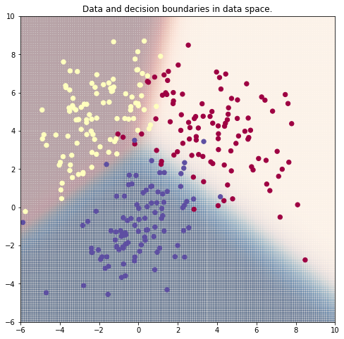
Literature
Licenses
Notebook License (CC-BY-SA 4.0)
The following license applies to the complete notebook, including code cells. It does however not apply to any referenced external media (e.g., images).
Automatic Differentiation for Matrices
by Christian Herta, Diyar Oktay
is licensed under a Creative Commons Attribution-ShareAlike 4.0 International License.
Based on a work at https://gitlab.com/deep.TEACHING.
Code License (MIT)
The following license only applies to code cells of the notebook.
Copyright 2019 Christian Herta, Diyar Oktay
Permission is hereby granted, free of charge, to any person obtaining a copy of this software and associated documentation files (the "Software"), to deal in the Software without restriction, including without limitation the rights to use, copy, modify, merge, publish, distribute, sublicense, and/or sell copies of the Software, and to permit persons to whom the Software is furnished to do so, subject to the following conditions:
The above copyright notice and this permission notice shall be included in all copies or substantial portions of the Software.
THE SOFTWARE IS PROVIDED "AS IS", WITHOUT WARRANTY OF ANY KIND, EXPRESS OR IMPLIED, INCLUDING BUT NOT LIMITED TO THE WARRANTIES OF MERCHANTABILITY, FITNESS FOR A PARTICULAR PURPOSE AND NONINFRINGEMENT. IN NO EVENT SHALL THE AUTHORS OR COPYRIGHT HOLDERS BE LIABLE FOR ANY CLAIM, DAMAGES OR OTHER LIABILITY, WHETHER IN AN ACTION OF CONTRACT, TORT OR OTHERWISE, ARISING FROM, OUT OF OR IN CONNECTION WITH THE SOFTWARE OR THE USE OR OTHER DEALINGS IN THE SOFTWARE.