
Automatic Differentiation for Scalars (Differentiable Programming)
Table of Contents
Introduction
In this notebook you will implement a Scalar class that supports automatic differentiation. Mostly, machine learning models correspond to mathematical functions that are composed by simple mathematical operators, e.g.,$ + $,$ * $ and$ .^2 $. So, the function can be represented by a computational graph.
For example the function$ f(x,y,z) = x + y * z $ can be represented by the following computional graph:
    y    z
     \  /
  x    *
    \ /
     +
     |
     f
The value of$ f $ can be computed for given values of$ x $,$ y $ and$ z $. Automatic differentiation is a procedure to compute the values of the derivatives of the output with repect to the inputs efficiently, i.e. here$ \frac{\partial f}{\partial x} $,$ \frac{\partial f}{\partial y} $ and$ \frac{\partial f}{\partial z} $ .
In the context of machine learning, we typically have:
-$ f $ is the cost function (including the machine learning model). So, we restrict ourself in the following to a scalar output of the computational graph.
- We want to compute the partial derivatives of the cost with respect to the parameters of the machine learning model.
Recap: In the introduction of machine learning you have learnt that "learning" is often minimizazion of the cost function on the training data set. We used gradient descent as optimization procedure.
Requirements
Knowledge
This notebook deals with computational graphs, the chain rule and backpropagation. A recommended read on the topic is
The Python implementation of the autodiff class is inspired by MXNet and discussed in-depth in the article
- Deep Learning Programming Style by Apache MXNet [AP17].
Python Modules
import numpy as np

from matplotlib import pyplot as plt
%matplotlib inline
Gradient Calculation by Backpropagation
Backpropagation (reverse mode automatic differentiation) is a method for efficient calculation of the gradient (and higher order derivatives).
If the (partial) derivative is defined for each operator, gradients of the computation graph can be computated automatically by backpropagation. The mathematical basis is the chain rule of calculus.
Gradient
The gradient $ grad $) of the (scalar) function$ f(.) $ with respect to (w.r.t.)$ \theta $ is the vector of the partial derivatives:
$ grad_\theta f(\theta)= \vec \nabla_\theta f(\theta) = \left( \begin{array}{c} \frac{\partial }{\partial \theta_1}\\ \frac{\partial }{\partial \theta_2}\\ \dots \\ \frac{\partial }{\partial \theta_n}\\ \end{array} \right)f(\theta) = \left( \begin{array}{c} \frac{\partial f(\theta)}{\partial \theta_1}\\ \frac{\partial f(\theta)}{\partial \theta_2}\\ \dots \\ \frac{\partial f(\theta)}{\partial \theta_n}\\ \end{array} \right) $
The principle idea of "reverse automatic differentiation" is to implement for each operator additionally how their derivative is computed. By the chain rule of calculus the individual derivatives of the operators are combined to computed the values of the wanted gradient, here$ \frac{\partial f}{\partial \theta_0} $,$ \frac{\partial f}{\partial \theta_1} $,$ \frac{\partial f}{\partial \theta_2} $ etc.
At the end of this notebook, we'll apply our autodiff class in a linear regression example and compute the gradients of the weight and bias using autodiff.
Math Recap: Chain Rule
Chain rule for a function$ c(b(w)) $ $ c $ is a function of$ b $ and$ b $ is a function of$ w $):
$ \frac{\partial c(b(w))}{\partial w} = \frac{\partial c(b(w))}{\partial b} \frac{\partial b(w)}{\partial w} $
Multivariable Chain Rule
$ \frac{\partial}{\partial t} f(x(t), y(t)) = \frac{\partial f}{\partial x} \frac{\partial x}{\partial t}+ \frac{\partial f}{\partial y}\frac{\partial y}{\partial t} $
If there are multiple paths to a parameter (here$ t $), we must add the partial derivatives ("the gradients").
Side Note: Total derivative vs partial derivative
For$ z = z(a, b) $ $ \frac{ d z}{d a} = \frac{\partial z}{\partial a} \frac{d a}{d a} + \frac{\partial z}{\partial b} \frac{d b}{d a} = \frac{\partial z}{\partial a} + \frac{\partial z}{\partial b} \frac{d b}{d a} $
if$ b $ is independent of$ a $, i.e.$ \frac{d b}{d a} = 0 $, we have:
$ \frac{ d z}{d a} = \frac{\partial z}{\partial a} + \frac{\partial z}{\partial b} \frac{d b}{d a} = \frac{\partial z}{\partial a} $
Sum and product rule
if$ b $ is not a function of$ u $:
$ \frac{ \partial (a b)}{\partial u} = \frac{\partial a}{\partial u} b + a \frac{\partial b}{\partial u} = \frac{\partial a}{\partial u} b $
$ \frac{ \partial (a(u) + b)}{\partial u} = \frac{\partial a}{\partial u} $
Backpropagation
We have a computational graph to compute$ c $ and two parameters in the graph$ v $ and$ w $. o1,o2 and o3 are arbitrary operators.
This is represented by the following computational graph:

We want to compute the two partial derivatives$ \frac{\partial c(b(a(w, v),y),z)}{\partial w} $ and$ \frac{\partial c(b(a(w, v),y),z)}{\partial v} $.
Note that the application of the chain rule results in: $ \frac{\partial c(b(a(w, v),y),z)}{\partial w} = \frac{\partial c(b,z)}{\partial b}\frac{\partial b(a,y)}{\partial a} \frac{\partial a(w,v)}{\partial w} $
$ \frac{\partial c(b(a(w, v),y),z)}{\partial v} = \frac{\partial c(b,z)}{\partial b}\frac{\partial b(a,y)}{\partial a} \frac{\partial a(w,v)}{\partial v} $
The first two factors of both expressions are the same. So, we need to compute them only once. That's the key idea of backpropagation. We need to compute such factors only once and can backpropagate them through the graph. This is much more efficient as to compute the partial derivatives independently.
Example for the given operator graph
Assume o1 and o3 are the multiplication operator $ * $) and o2 is an add-operator $ + $).
Note that the application of the chain rule results in:
$ \frac{\partial c}{\partial w} = \frac{\partial c(b,z)}{\partial b}\frac{\partial b}{\partial w} = \frac{\partial (z * b)}{\partial b}\frac{\partial b}{\partial w} = z \frac{\partial b}{\partial w} $
$ \frac{\partial b}{\partial w} = \frac{\partial b(a,y)}{\partial w} = \frac{\partial b(a,y)}{\partial a} \frac{\partial a}{\partial w}= \frac{\partial (a+y)}{\partial a} \frac{\partial a}{\partial w} = 1 \frac{\partial a}{\partial w} $
$ \frac{\partial a}{\partial w} = \frac{\partial a(wv)}{\partial w} = \frac{\partial a(wv)}{\partial w} = v $
so we have:
$ \frac{\partial c}{\partial w} = z * 1 * v = z * v $
For$ \frac{\partial c}{\partial v} $ the first to factors of the chain rule $ \frac{\partial c}{\partial b} = z $ and$ \frac{\partial b}{\partial a} = 1 $) are the same and we can reuse them:
$ \frac{\partial c}{\partial v} = z * 1 * \frac{\partial a(w,v)}{\partial w} = z * 1 * w = z * w $
Exercises
Compute the derivatives (pen & paper)
Consider the function $ E = (w_1 \cdot x_1 + w_2 \cdot x_2) \cdot (w_3 \cdot x_3) = h \cdot g $
with
$ h = (w_1 \cdot x_1 + w_2 \cdot x_2) $
$ g = (w_3 \cdot x_3) $
Compute the partial derivative of$ E $ with respect to each of the weights:
-$ \frac{\partial E}{\partial w_1} $
-$ \frac{\partial E}{\partial w_2} $
-$ \frac{\partial E}{\partial w_3} $
Note:
In general for a Product-Node$ g \cdot h $: The factor$ g $ flows back in the graph into the$ h $-Branch for computing all derivatives$ \frac{\partial E}{\partial w_i} $ in the$ h $-Branch. So, we need first to compute$ g $ in a forward pass to get the$ g $ value. Then in the backward pass, we can propagate the$ g $ values back through the$ h $ branch to compute all derivatives on the$ h $ branch$ \frac{\partial E}{\partial w_i} $.
So, in general we must first compute a forward pass to get all values of all nodes. We often need the values to compute the derivatives at a node.
def round_and_hash(value, precision=4, dtype=np.float32):
    """
    Function to round and hash a scalar or numpy array of scalars.
    Used to compare results with true solutions without spoiling the solution.
    """
    rounded = np.array([value], dtype=dtype).round(decimals=precision)
    hashed = hashlib.md5(rounded).hexdigest()
    return hashed
Exercise: Pen and Paper Backpropagation
Given the function$ f(a,b,c) $ as a computational graph with the following values for the parameters:
$ a = 2 \\ b = e \; (Euler \;number, \;b \approx 2.7183) \\ c = 3 $

Tasks:
- Give an equation (inline) that expresses the graph.
- Calculate the partial derivatives$ \frac {\partial out} {\partial a} $,$ \frac {\partial out} {\partial b} $. and$ \frac {\partial out} {\partial c} $ using calculus on pen & paper by using the backprop procedure.
- For$ b $ use the the true$ Euler \;number $ and not the approximation
- Assign your results to variables
partial_a,partial_bandpartial_cto verify your solution with the software test below
Note: The node$ 1/x $ computes the inverse of the input$ x $, i.e. the output is$ 1/x $ or$ x^{-1} $
partial_a = None ### assign what you have calculated
partial_b = None ### assign what you have calculated
partial_c = None ### assign what you have calculated
# Test of your solution
assert round_and_hash(partial_a) == '2fb0a82d3fe965c8a0d9ce85970058d8'
assert round_and_hash(partial_b) == 'b6bfa6042c097c90ab76a61300d2429a'
assert round_and_hash(partial_c) == '2fb0a82d3fe965c8a0d9ce85970058d8'Autodiff class Scalar
Deep learning frameworks support automatic differentiation via backpropagation through the computational graph.
To demonstrate how autodiff works we implement a simple autodiff python class Scalar. For each operator we have to implement additionally how the operator is differentiated. Therefore each operator has a grad-function.
Note: We have to add multiple path to the same variable as the multivariable chain rule (see above) tells us.
In the implementation we store the partial derivatives in a python dictionary.
We need a helper function combine_dicts for taking the multivariate chain rule into account:
import operator
def combine_dicts(a, b, op=operator.add):
    x = (list(a.items()) + list(b.items()) +
        [(k, op(a[k], b[k])) for k in set(b) & set(a)])
    return {x[i][0]: x[i][1] for i in range(0, len(x))}
# Here you see how `combine_dicts` work
a = {'a': 2, 'b':3, 'c':4}
b = {'a': 5, 'c':6, 'x':7}
combine_dicts(a, b)# and another example
A = {'a':-1.3, 'b':-4, 'c':3}
B = {'b':3, 'c':4, 'd':5}
combine_dicts(A,B)class Scalar(object): # same as Node() class in the video
"""Simple Scalar object that supports autodiff."""
def __init__(self, value, name=None):
self.value = value
if name: # we want only the partial derivatives w.r.t. scalar instances which have a name.
self.grad = lambda g : {name : g}
else:
self.grad = lambda g : {}
def __add__(self, other):
assert isinstance(other, Scalar)
# forward pass: addition is simple:
ret = Scalar(self.value + other.value)
def grad(g): # g is the backpropagated value
x = self.grad(g * 1) # we put the `* 1` to make it more clear: d(a+b)\da = 1
x = combine_dicts(x, other.grad(g * 1))
return x
ret.grad = grad
return ret
# Forward pass
a = Scalar(3., 'a')
b = Scalar(2., 'b')
d = Scalar(4.)

c = b + a
e = d + c
e.value
# but we also have the intermediate values, e.g.
d.value# backward pass
derivatives = e.grad(1)
derivativesLet's try and get a better understanding of what happens in the add function by looking at an example of one operation. Node A and B are two scalar values. Node C is then constructed through the statement C = A + B, which is equivalent to both C = A.__add__(B) and C = Scalar.__add__(A,B)

root is the output of the complete computational graph.
- In the
__add__function, nodeAis stored inselfand node B is stored inother. The node C which is being created is stored inret. - The derivatives of$ C=C(A,B) $ with respect to its inputs are$ \frac{\partial C}{\partial A} = 1 $ and$ \frac{\partial C}{\partial B} = 1 $
-
What about the argument
g?gis the total backpropagated value so far. So, it's the partial derivative of the output of the computational graph with respect to C, let's call it$ \frac{\partial root}{\partial C} $ . The chain rule tells us to get the value of the entire computational graph with respect toAandB, we multiply this value with the current branch respectively. I.e. $ \frac{\partial root}{\partial A} = \frac{\partial root}{\partial C} * \frac{\partial C}{\partial A} = g * \frac{\partial C}{\partial A} $$ \frac{\partial root}{\partial B} = \frac{\partial root}{\partial C} * \frac{\partial C}{\partial B} = g * \frac{\partial C}{\partial B} $
- We pass the value$ g * 1 $ or just$ g $ to the grad function of both
AandB. We use thecombine_dictshelper to produce the joined dictionary { 'A' :$ \frac{\partial root}{\partial A} $ , 'B' :$ \frac{\partial root}{\partial B} $ } ifAandBare named input nodes in the computational graph.
Task: Implement the multiplication and square $ ^2 $) operators.
def __mul__(self, other):
    assert isinstance(other, Scalar)
    raise NotImplementedError()


def square(self):
    assert isinstance(other, Scalar)
    raise NotImplementedError()

Scalar.__mul__ = __mul__
Scalar.square = square
Example: A computational graph using autodiff
Consider this computational graph.
 $ g $ is the backpropagated "gradient value" - in general it is different at each position. It starts at the root of the tree with$ g = 1 $ $ \frac{\partial root}{\partial root} = 1 $).
Example: $ d = (a * b) + 1 $
$ \frac{\partial d}{\partial a} = \frac{\partial (a*b+1)}{ \partial a} = b $
$ \frac{\partial d}{\partial b} = \frac{\partial (a*b+1)}{ \partial b} = a $
In Python code using our autodiff Scalar class, we can construct the graph above
dynamically via the actual forward computation. That is called Define-by-Run.
Then, we can compute the derivatives by calling grad(1) on the output of the graph.
# Chain basic operations to construct a graph
a = Scalar(1., 'a')
b = Scalar(2., 'b')
c = b * a
d = c + Scalar(1.)

# Compute the derivatives of d with respect to a and b
derivatives = d.grad(1)
derivatives
Verify your implementation: You can run the following tests to test if your implementation is working as expected
# test forward pass of multiplication
assert d.value == 3.

# test backward path of multipication
assert d.grad(1)['a']==2.0
assert d.grad(1)['b']==1.0
a = Scalar(1., 'a')
b = Scalar(3., 'b')
c = b.square() * a
d = (c + Scalar(1.)).square()
# test forward pass
assert d.value == 100.# test backward pass
assert d.grad(1)['a'] == 180
assert d.grad(1)['b'] == 120Exercise: Linear Regression using autodiff
In this exercise, you have to implement Linear Regression as a non-trivial example to show how the autodiff class can be used.
# generate some train data
x_min = -10.
x_max = 10.
m = 10

x = np.random.uniform(x_min, x_max, m)
a = 10.
c = 5.
y_noise_sigma = 3.
y = a + c * x + np.random.randn(len(x)) * y_noise_sigmaplt.plot(x, y, "bo")
plt.xlabel("x")
plt.ylabel("y")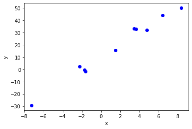
Task: Implement and apply linear regression
In the following task, you have to implement linear regression using the Scalar class.
- Implement the linear model and the cost function using the
Scalarclass. For the cost function you have to loop over the complete training data set.Scalardon't allow any vectorized implementation. So each$ x^{(i)} $ and each$ y^{(i)} $ becomes a node in the computational graph. Use the given training data stored inxandy.
The linear model is:
$ h(x^{(i)}) = b + x^{(i)} * w $
- with an input$ x^{(i)} $ with bias$ b $ and weight$ w $.$ b $ and$ w $ are the parameters of the model.
The mean-squared-error cost is the sum over$ m $ samples with ground truth data values$ y^{(i)} $:
$ cost =\frac{1}{m}\sum_{i=1}^{m}{(h(x^{(i)})-y^{(i)})^2} $
-
Implement gradient descent and train the model with the data. You can compute the derivatives of the cost function with a single call
cost.grad(1). The value$ 1 $ is backpropagated through the graph and you obtain the derivatives of the cost w.r.t the weight$ \frac{\partial{cost}}{\partial w} $ and w.r.t to the bias$ \frac{\partial{cost}}{\partial b} $. Use these derivatives in gradient descent to optimize the model. -
Plot
-
the training progress and
-
fitted model with the data
to show that your implementation works. The result should look like this:


Literature
Licenses
Notebook License (CC-BY-SA 4.0)
The following license applies to the complete notebook, including code cells. It does however not apply to any referenced external media (e.g., images).
Automatic Differentiation for Scalars
by Christian Herta
is licensed under a Creative Commons Attribution-ShareAlike 4.0 International License.
Based on a work at https://gitlab.com/deep.TEACHING.
Code License (MIT)
The following license only applies to code cells of the notebook.
Copyright 2019 Christian Herta
Permission is hereby granted, free of charge, to any person obtaining a copy of this software and associated documentation files (the "Software"), to deal in the Software without restriction, including without limitation the rights to use, copy, modify, merge, publish, distribute, sublicense, and/or sell copies of the Software, and to permit persons to whom the Software is furnished to do so, subject to the following conditions:
The above copyright notice and this permission notice shall be included in all copies or substantial portions of the Software.
THE SOFTWARE IS PROVIDED "AS IS", WITHOUT WARRANTY OF ANY KIND, EXPRESS OR IMPLIED, INCLUDING BUT NOT LIMITED TO THE WARRANTIES OF MERCHANTABILITY, FITNESS FOR A PARTICULAR PURPOSE AND NONINFRINGEMENT. IN NO EVENT SHALL THE AUTHORS OR COPYRIGHT HOLDERS BE LIABLE FOR ANY CLAIM, DAMAGES OR OTHER LIABILITY, WHETHER IN AN ACTION OF CONTRACT, TORT OR OTHERWISE, ARISING FROM, OUT OF OR IN CONNECTION WITH THE SOFTWARE OR THE USE OR OTHER DEALINGS IN THE SOFTWARE.