
Image Classification - Softmax Regression
Table of Contents
- Introduction
- Load, Explore and Prepare Dataset
- Exercises
- Plot Digits
- Preparation of Train- and Test-Split
- Define a Linear Classifier Using Softmax
- Reduce the Cost Using Gradient Descent
- Stochastical Gradient Descent
- Evaluate the Vanilla Gradient Descent Model
- Evaluate the Stochastical Gradient Descent Model
- Appendix
- Predicting an Own Example
- Preparation
- Creating an Own Batch
- Evaluation
- Normalize our Images
- Evaluation
- Summary and Outlook
- Literature
- Licenses
Introduction
In this exercise you will learn how to classify images of handwritten digits. For classification you will implement the logistic regression, or better said, as we have more than two classes, softmax regression. Further you will learn about stochastic gradient descent (opposed to gradient descent) and for evaluation of your model, the accuracy and f1-score.
Requirements
Knowledge
Required knowledge:
- Machine learning models linear models
- Gradient descent.
- Softmax
Literature:
- Lecture Notes of CS231n: Linear classification: Support Vector Machine, Softmax .
- Eli Bendersky blog post about Softmax and its derivative.
Python Modules
With the deep.TEACHING convention, all python modules needed to run the notebook are loaded centrally at the beginning.
# All necessary imports at the beginning
import numpy as np
import matplotlib.pyplot as plt
import matplotlib.image as mpimg
import os
import shutil
import gzip
import urllib.request
import pandas as pd
Load, Explore and Prepare Dataset
The MNIST dataset is a classic Machine Learning dataset you can get it and more information about it from the website of Yann Lecun. MNIST contains handwrittin digits and is split into a trainings set of 60000 examples and a test set of 10000 examples. You can use the module sklearn to load the MNIST dataset in a convenient way.
easy load, mldata.org, orginal mnist, mnist link and description
Note:
If the cells below throws an error, the problem might be a broken download link. In that case, download the dataset from another source, e.g. from https://www.kaggle.com/avnishnish/mnist-original, and unzip it and place it under BASE_DATA_DIR.
BASE_DATA_DIR = os.path.expanduser('~/deep.TEACHING/data')

class Mnist:
    """Downloads, loads into numpy array and reshapes the common machine learning dataset: MNIST

    The MNIST dataset contains handwritten digits, available from http://yann.lecun.com/exdb/mnist/,
    has a training set of 60,000 examples, and a test set of 10,000 examples. With the class you can
    download the dataset and prepare them for usage, e.g., flatten the images or hot-encode the labels.
    """

    def __init__(self, data_dir=None, auto_download=True, verbose=True):
        """Downloads and moves MNIST dataset in a given folder.

        MNIST will be downloaded from http://yann.lecun.com/exdb/mnist/ and moved
        into the folder 'data_dir', if a path is given by the user, else files
        will be moved into a folder specified by the deep-teaching-commons
        config file.

        Args:
            data_dir: A string representing a path where you want to store MNIST.
            auto_download: A boolean, if True and the given 'data_dir' does not exists, MNIST will be download.
            verbose: A boolean indicating more user feedback or not.
        """
        self.data_dir = data_dir
        self.verbose = verbose

        if self.data_dir is None:
            self.data_dir = os.path.join(BASE_DATA_DIR, 'MNIST')

        self.data_url = 'http://yann.lecun.com/exdb/mnist/'
        self.files = ['train-images-idx3-ubyte.gz','train-labels-idx1-ubyte.gz','t10k-images-idx3-ubyte.gz', 't10k-labels-idx1-ubyte.gz']

        if auto_download:
            if self.verbose:
                print('auto download is active, attempting download')
            self.download()

    def download(self):
        """Downloads MNIST dataset.

        Creates a directory, downloads MNIST and moves the data into the
        directory. MNIST source and target directory are defined by
        class initialization (__init__).

        TODO:
            Maybe redesign so it can be used as standalone method.
        """
        if os.path.exists(self.data_dir):
            if self.verbose:
                print('mnist data directory already exists, download aborted')
        else:
            if self.verbose:
                print('data directory does not exist, starting download...')
            # Create directories
            os.makedirs(self.data_dir)
            # Download each file and move it to given self.data_dir
            for file in self.files:
                urllib.request.urlretrieve(self.data_url + file, file)
                shutil.move(file, os.path.join(self.data_dir, file))
                if self.verbose:
                        print(file,'successfully downloaded')
            if self.verbose:
                print('... mnist data completely downloaded, enjoy.')

    def get_all_data(self, one_hot_enc=None, flatten=True, normalized=None):
        """Loads MNIST dataset into four numpy arrays.

        Default setup will return training and test images in a flat resprensentaion,
        meaning each image is row of 28*28 (784) pixel values. Labels are encoded as
        digit between 0 and 9. You can change both representation using the arguments,
        e.g., to preserve the image dimensions.

        Args:
            one_hot_enc (boolean): Indicates if labels returned in standard (0-9) or one-hot-encoded form
            flatten (boolean): Images will be returned as vector (flatten) or as matrix
            normalized (boolean): Indicates if pixels (0-253) will be normalized

        Returns:
            train_data (ndarray): A matrix containing training images
            train_labels (ndarray): A vector containing training labels
            test_data (ndarray): A matrix containing test images
            test_labels (ndarray): A vector containing test labels
        """
        train_images = self.get_images(os.path.join(self.data_dir,self.files[0]))
        train_labels = self.get_labels(os.path.join(self.data_dir,self.files[1]))
        test_images = self.get_images(os.path.join(self.data_dir,self.files[2]))
        test_labels = self.get_labels(os.path.join(self.data_dir,self.files[3]))

        if one_hot_enc:
            train_labels, test_labels = [self.to_one_hot_enc(labels) for labels in (train_labels, test_labels)]

        if flatten is False:
            train_images, test_images = [images.reshape(-1,28,28) for images in (train_images, test_images)]

        if normalized:
            train_images, test_images = [images/np.float32(256) for images in (train_images, test_images)]

        return train_images, train_labels, test_images, test_labels

    def get_images(self, file_path):
        """Unzips, reads and reshapes image files.

        Args:
            file_path (string): mnist image data file

        Returns:
            ndarray: A matrix containing flatten images
        """
        with gzip.open(file_path, 'rb') as file:
            images = np.frombuffer(file.read(), np.uint8, offset=16)
        return images.reshape(-1, 28 * 28)

    def get_labels(self, file_path):
        """Unzips and read label file.

        Args:
            file_path (string): mnist label data file

        Returns:
            ndarray: A vector containing labels
        """
        with gzip.open(file_path, 'rb') as file:
            labels = np.frombuffer(file.read(), np.uint8, offset=8)
        return labels


    def to_one_hot_enc(self, labels):
        """Converts standard MNIST label representation into an one-hot-encoding.

        Converts labels into a one-hot-encoding representation. It is done by
        manipulating a one diagonal matrix with fancy indexing.

        Args:
            labels (ndarray): Array of mnist labels

        Returns:
            ndarray: A matrix containing a one-hot-encoded label each row

        Example:
            [2,9,0] --> [[0,0,1,0,0,0,0,0,0,0]
                         [0,0,0,0,0,0,0,0,0,1]
                         [1,0,0,0,0,0,0,0,0,0]]
        """
        return np.eye(10)[labels]
mnist = Mnist()
X_train_, y_train, X_test_, y_test = mnist.get_all_data(one_hot_enc=True, flatten=True)
auto download is active, attempting download
mnist data directory already exists, download aborted
# for the Bias-Trick: add a one column at the beginning of the data matricies
M_train = X_train_.shape[0]
X_train = np.concatenate((np.ones((M_train, 1)), X_train_), axis=1)
M_test = X_test_.shape[0]
X_test = np.concatenate((np.ones((M_test, 1)), X_test_), axis=1)
Task
Explain the bias trick.
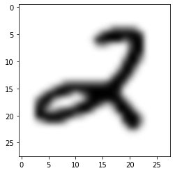
To get a visualization of MNIST we will plot a digit. Each line represents an image in flatten form (all pixel in a row). We have change the shape from a vector back to a matrix of the original shape to plot the image. In the case of MNIST this means a conversion of 784 pixel into 28x28 pixel. In addition we will check the label of that digit to verify it correspond to the image.
def plot_mnist_digit(digit):
    image = digit.reshape(28, 28)
    plt.imshow(image, cmap='binary', interpolation='bicubic')

#choose a random number, plot it and check label
random_number = np.random.randint(1,len(X_train)-1)
print('label:',y_train[random_number])
plot_mnist_digit(X_train_[random_number])
label: [0. 0. 0. 1. 0. 0. 0. 0. 0. 0.]
Exercises
Plot Digits
After a glimpse into MNIST let us explore it a bit further.
Task:
Write a function plot_mnist_digits(data, examples_each_row) that plots configurable number of examples for each class, like:

def plot_mnist_digits(X, y, examples_each_row):
    ############################################
    #TODO: Write a function that plots as many #
    #      examples of each class as defined   #
    #      by 'examples_each_row'              #
    ############################################

    pass
    #raise NotImplementedError()


    ############################################
    #             END OF YOUR CODE             #
    ############################################

plot_mnist_digits(X_train, y_train, examples_each_row=10)
Preparation of Train- and Test-Split
After exploring MNIST let us prepare the date for our linear classifier. First we will shuffle the training data to get a random distribution.
# shuffle training data
shuffle_index = np.random.permutation(len(X_train))
X_train, y_train = X_train[shuffle_index], y_train[shuffle_index]
Define a Linear Classifier Using Softmax
Softmax Regression Model
First a linear transformation of the data is performed to calculate the logits or score values (before softmax). Note that$ \vec f $ is a vector.
$ \vec f(\vec x) = \vec x^T \cdot \Theta $ with -$ \vec x^{(m)} $ is the$ m $-th training image (as vector).$ \vec x_0^{(m)}=1 $ is an additional bias. -$ K $ is the number of classes (10 for MNIST) and$ k $ is the class index. -$ M $ is the number of training examples. -$ N $ is the number of features (image pixels). -$ \Theta $: Parameter matrix with$ N+1 $ rows and$ K $ columns.
Each element$ f_k $ of$ \vec f(\vec x) $ is the logit value of the$ k $-th class. So,$ f_{y^{(m)}}(\vec x^{(m)}) $ is the logit value of the label class$ y^{(m)} $ for image$ \vec x^{(m)} $.
From$ \vec f $ the prediction probabilities are computed by softmax:
$ \vec h(\vec x) = \text{softmax} (\vec f ( \vec x )) $
The elements of$ \vec h $ are$ h_k(\vec x) $. $ h_k(\vec x) $ are the predicted probabilities that$ \vec x $ belongs to class$ k $:
$ h_k(\vec x) = p( \text{class} = k \mid \vec x; \Theta) $
So, $ h_{y^{(m)}}(\vec x) = \frac{ \exp\left({f_{y^{(m)}}(\vec x^{(m)}; \Theta)}\right)}{\sum_{k=1}^{K}\exp\left({f_k(\vec x^{(m)}; \Theta)}\right)} $ is the predicted probability for the label class of image$ m $:
Tasks
Answer the following questions about softmax :
- What is the range (possible values) of the softmax function?
- What is the sum of all softmax outputs?
- Assume the logit of output$ k $ is increased a little bit (the other logits stay constant). How changes the softmax of output$ k $? How change the other softmax outputs?
Cost function
We will train a model to classify the MNIST dataset with the following equation for the cost function (loss):
$ J(\Theta) = \frac{1}{M} \sum_{m=1}^{M} - \log\; \frac{ \exp\left({f_{y^{(m)}}(\vec x^{(m)}; \Theta)}\right)}{\sum_{k=1}^{K}\exp\left({f_k(\vec x^{(m)}; \Theta)}\right)} + \lambda \sum_{k=1}^{K}\sum_{n=1}^{N} \Theta_{nk}^2 \label{eq:cost_function} \tag{1} $
with -$ J(\Theta) $: Cost function (also called loss$ L $)
Tasks
Answer the following questions about the cost function:
- What is the meaning of the first term of equation$ \eqref{eq:cost_function} $? $ \frac{1}{M} \sum_{m=1}^{M} - \log\; \frac{ \exp\left({f_{y^{(m)}}(\vec x^{(m)}; \Theta)}\right)}{\sum_{k=1}^{K}\exp\left({f_k(\vec x^{(m)}; \Theta)}\right)} $
-
What is the meaning of the second term of equation$ \eqref{eq:cost_function} $? $ \frac{\lambda}{2} \sum_{k=1}^{K}\sum_{n=1}^{N} \Theta_{nk}^2 $ What is the function of this term?
-
How many parameters$ Q $ has the matrix$ \Theta $? Note: Don't forget the bias terms.
-
Explain why `DOUBLE
- \log\; \frac{ \exp\left({f{y^{(m)}}(\vec x^{(m)}; \Theta)}\right)}{\sum{k=1}^{K}\exp\left({f_k(\vec x^{(m)}; \Theta)}\right)}
DOUBLE
is equivalent toDOUBLE - {f{y^{(m)}}(\vec x^{(m)}; \Theta)} + \log \sum{k=1}^{K}\exp\left({f_k(\vec x^{(m)}; \Theta)}\right) DOUBLE`
- For the gradient descent implementation (see below) we need the gradient. Show that the components of the gradient are
$ \frac{\partial \log h_k(\vec x, \Theta)}{\partial \Theta_{ni}} = \left(\delta_{ki} - \text{softmax}_i(\vec f(\vec x))\right) x_n $
Hint: Use the chain rule:
DOUBLE \frac{\partial \log h_k}{\partial \Theta_{ni}} = \frac{\partial \log h_k}{\partial f_j}\frac{\partial f_j}{\partial \Theta_{ni}} DOUBLE``SINGLE \delta_{ki} SINGLEis the Kronecker Delta, i.e. -$ \delta_{ki}=1 $, if$ k=i $ -$ \delta_{ki}=0 $, if$ k\neq i $
Side Note: Probabilistic interpretation
Note that $ h_k(\vec x; \Theta) = p( k \mid \vec x; \Theta) $
with -$ p( k \mid \vec x; \Theta) $ predicted probability that image$ \vec x $ belongs to class$ k $.
So, $ \begin{align} J(\Theta) &= \frac{1}{M} \sum_{m=1}^{M} - \log\; \frac{ \exp\left({f_{y^{(m)}}(\vec x^{(m)}; \Theta)}\right)}{\sum_{k=1}^{K}\exp\left({f_k(\vec x^{(m)}; \Theta)}\right)} + \frac{\lambda}{2} \sum_{k=1}^{K}\sum_{n=1}^{N} \Theta_{nk}^2 \\ &= \frac{1}{M} \sum_{m=1}^{M} L^{(m)} + \frac{\lambda}{2} \sum_{k=1}^{K}\sum_{n=1}^{N} \Theta_{nk}^2 \end{align} $
`DOUBLE L^{(m)} =
- \log\; \frac{ \exp\left({f{y^{(m)}}(\vec x^{(m)}; \Theta)}\right)}{\sum{k=1}^{K}\exp\left({fk(\vec x^{(m)}; \Theta)}\right)}=- \log h{y^{(m)}}(\vec x; \Theta) = - \log p( y^{(m)} \mid \vec x; \Theta) DOUBLE`
-$ L^{(m)} $ seen as a function of$ \Theta $ is (point-wise) negative log-likelihood.
Using the universal equation for the cost function we can see the separate parts of that hugh equation.
$ J(\Theta) = \frac{1}{M} \sum_i L^{(m)} + \lambda R(\Theta) $
We will implement each part on its own and put them together. That way it is much easier to understand whats going on.
Task:
Let us start with the logits / class scores:
$ F(X;\Theta) = X \cdot \Theta $
It is possible to calculate all score values with one matrix multiplication (dot product). So, we can use the whole training data$ X $ instead of one digit image$ \vec x^{(m)} $. With the numpy dot product it's much faster than using python loops.
def class_scores(X, theta):
    ############################################
    #TODO: Implement the hypothesis and return #
    #      the score values for each class of  #
    #      every digit.                        #
    ############################################
    raise NotImplementedError()
    ############################################
    #             END OF YOUR CODE             #
    ############################################
First, let's implement the data dependent loss$ L^{(m)} $.
Note, that y_train is one hot encoded.
y_train[:3]Task:
Implement the functions softmax and data_loss.
softmaxcalculates the prediction probabilities $ h_k(\vec x; \Theta) $) from the class scores$ f_k(\vec x; \Theta) $ for a whole (mini-)batch, e.g.$ H(X;\Theta) $ from$ F(X;\Theta) $. The output is an 2-D numpy array with shape (M,K).
data_losscalculates the$ L^{(m)} $ for a whole (mini-)batch. The output is an numpy array with shape (M,), i.e. the$ L^{(m)} $ are the elements of the 1-D array.
Hint:
The correct classes (labels) are in a one hot encoding shape, so you can use a matrix multiplication to extract the correct class.
# Calculate class probability distribution for each digit from given class scores
def softmax(class_scores):
    ############################################
    #TODO: Use the softmax function to compute #
    #      class probabilties                  #
    ############################################
    raise NotImplementedError()
    ############################################
    #             END OF YOUR CODE             #
    ############################################

# Compute data_loss L_i for the correct class
def data_loss(class_probabilities, onehot_encode_label):
    ############################################
    #TODO: With hot encoded labels and class   #
    #      probabilties calculate data loss    #
    #      L_i                                 #
    ############################################
    raise NotImplementedError()
    ############################################
    #             END OF YOUR CODE             #
    ############################################
Now, we will calculate the total cost$ J(\Theta) $ using the defined functions.
$ J(\Theta) = \frac{1}{M} \sum_m L^{(m)} + \lambda R(\Theta) $
We will have to calculate the gradient for our cost function$ J $ with the aim to minimize the cost.
$ {\displaystyle \operatorname {grad} (J(\Theta))= \vec \nabla J(\Theta)={\begin{pmatrix}{\frac {\partial J(\Theta)}{\partial \theta_{1}}}\\\vdots \\{\frac {\partial J(\Theta)}{\partial \theta_{Q}}}\end{pmatrix}}.} $
- The total number of parameters is$ Q = K (N+1) $
Task:
Implement the total cost (total_cost).
def total_cost(X, Y, theta, lambda_):
    # X is the design (data) matrix
    # Y are the targets one hot encoded.
    # theta are the parameter as matrix
    # lambda_ is a hyperparameter for the regularization strength

    H = softmax(class_scores(X,theta))
    loss_Lm = data_loss(probabilities, encoded_labels)


    ############################################
    #TODO: Put everthing together and calculate #
    #      the total cost with given            #
    #      variables.                           #
    ############################################
    raise NotImplementedError()

    ############################################
    #             END OF YOUR CODE             #
    ############################################
Pen and Paper task
Show that from $ \Theta_{nk}^{new} \leftarrow \Theta_{nk}^{old} - \frac{\alpha}{M} \sum_{m=1}^M \frac{\partial \log h_{y^{(m)}}(\vec x^{(m)}, \Theta^{old})}{\partial \Theta_{nk}} = \Theta_{nk}^{old} - \frac{\alpha}{M}\left( \sum_{m=1}^M\left( \text{softmax}_k(\vec f(\vec x^{(m)}; \Theta^{old})) - \delta_{{y^{(m)}}k} \right) x_n^{(m)} \right) $
follows (for our batch implementation) of gradient descent (without the regularization term!):
$ \Theta^{new} \leftarrow \Theta^{old} - \frac{\alpha}{M} \left( X^T \cdot (H-Y^{OH}) \right) $
-$ H $ is the softmax output as matrix with shape (M, K). -$ Y_{OH} $ are the targets one-hot encoded.$ Y_{OH} $ has shape (M, K). -$ X $ is the data matrix with shape (M, N+1) (bias units added).
Implementation task
Implement the gradient-function:
def gradient(X, Y, theta, lambda_):

    H = softmax(class_scores(X, theta))

    ############################################
    #TODO: Put everthing together and calculate #
    #      the gradient with given              #
    #      variables.                           #
    #############################################
    raise NotImplementedError()

    ############################################
    #             END OF YOUR CODE             #
    ############################################
Reduce the Cost Using Gradient Descent
Gradient descent is a way to minimize our Loss functions. It iteratively moves toward a set of parameter values that minimize our Loss function. This iterative minimization is achieved using calculus, taking steps in the negative direction of the gradient (which is a vector that shows us the highest rise).
$ {\displaystyle \vec {\theta} _{new}=\vec {\theta} _{old}- \alpha \cdot \vec \nabla J(\Theta)} $
with -$ \alpha $: learning rate -$ \vec \theta $ is the "vectorized" version of all parameters$ \Theta $ (Not used directly in implementation).
$ {\displaystyle {\begin{pmatrix} \theta_1 \\\vdots \\ \theta_Q \end{pmatrix}}_{new} = {\begin{pmatrix} \theta_1 \\\vdots \\ \theta_Q \end{pmatrix}}_{old} -\alpha \space {\begin{pmatrix}{\frac {\partial L}{\partial \theta_{1}}}\\\vdots \\{\frac {\partial L}{\partial \theta_{Q}}}\end{pmatrix}}.} $
def gradient_descent(training_data, training_label, theta, lambda_=0.5, iterations=100, learning_rate=1e-5):
    losses = []

    for i in range(iterations):
        loss = total_cost(training_data, training_label, theta, lambda_)
        grad = gradient(training_data, training_label, theta, lambda_)
        losses.append(loss)
        theta -= (learning_rate * grad)
        print('epoch ', i, ' - cost ', loss)

    return theta, losses

# Initialize learnable parameters theta
theta = np.zeros([X_train.shape[1], len(y_train[0])])
# Start optimization with training data, theta and optional hyperparameters
opt_theta, loss_history = gradient_descent(X_train, y_train, theta, iterations=150)
epoch 0 - cost 2.3025850929940437
epoch 1 - cost 1.7197897851355572
epoch 2 - cost 1.387485258940546
epoch 3 - cost 1.1929807653996316
epoch 4 - cost 1.0868315460700073
epoch 5 - cost 0.9945089665450335
epoch 6 - cost 0.9695409713501421
epoch 7 - cost 0.8473984293629602
epoch 8 - cost 0.8234311786304473
epoch 9 - cost 0.7673577315626103
epoch 10 - cost 0.752781368811333
epoch 11 - cost 0.7033928420297415
epoch 12 - cost 0.6864613136856771
epoch 13 - cost 0.6538235456234421
epoch 14 - cost 0.637204605670394
epoch 15 - cost 0.6151595630022962
epoch 16 - cost 0.6005959137029724
epoch 17 - cost 0.5852636364046391
epoch 18 - cost 0.573317563047066
epoch 19 - cost 0.5620636975816435
epoch 20 - cost 0.5524483890101036
epoch 21 - cost 0.5436879596788453
epoch 22 - cost 0.5358468786084982
epoch 23 - cost 0.5286794103483146
epoch 24 - cost 0.5221030465038602
epoch 25 - cost 0.5160129505540578
epoch 26 - cost 0.5103399696826503
epoch 27 - cost 0.5050270793065171
epoch 28 - cost 0.5000307753876171
epoch 29 - cost 0.4953164802487935
epoch 30 - cost 0.49085630451321877
epoch 31 - cost 0.48662705615974344
epoch 32 - cost 0.48260902416428125
epoch 33 - cost 0.4787850760980687
epoch 34 - cost 0.4751401250613091
epoch 35 - cost 0.47166073447751233
epoch 36 - cost 0.4683348624972795
epoch 37 - cost 0.4651516593743792
epoch 38 - cost 0.46210131510484126
epoch 39 - cost 0.4591749311461999
epoch 40 - cost 0.45636441442567094
epoch 41 - cost 0.45366238586942004
epoch 42 - cost 0.4510621019448033
epoch 43 - cost 0.44855738634109815
epoch 44 - cost 0.44614257049929645
epoch 45 - cost 0.44381244152037486
epoch 46 - cost 0.4415621964508186
epoch 47 - cost 0.43938740201674775
epoch 48 - cost 0.4372839590694888
epoch 49 - cost 0.4352480711015146
epoch 50 - cost 0.43327621629738733
epoch 51 - cost 0.43136512266071153
epoch 52 - cost 0.4295117458266391
epoch 53 - cost 0.4277132492248859
epoch 54 - cost 0.4259669863056265
epoch 55 - cost 0.42427048458029953
epoch 56 - cost 0.42262143126307244
epoch 57 - cost 0.42101766032728144
epoch 58 - cost 0.419457140815523
epoch 59 - cost 0.41793796626287194
epoch 60 - cost 0.41645834511051405
epoch 61 - cost 0.4150165920024062
epoch 62 - cost 0.4136111198707294
epoch 63 - cost 0.4122404327273154
epoch 64 - cost 0.4109031190880527
epoch 65 - cost 0.409597845965837
epoch 66 - cost 0.4083233533750688
epoch 67 - cost 0.40707844929715953
epoch 68 - cost 0.4058620050621892
epoch 69 - cost 0.40467295110678997
epoch 70 - cost 0.4035102730726861
epoch 71 - cost 0.4023730082141267
epoch 72 - cost 0.4012602420858181
epoch 73 - cost 0.4001711054859114
epoch 74 - cost 0.3991047716312361
epoch 75 - cost 0.3980604535442704
epoch 76 - cost 0.3970374016334132
epoch 77 - cost 0.3960349014499212
epoch 78 - cost 0.3950522716065354
epoch 79 - cost 0.39408886184422537
epoch 80 - cost 0.3931440512348025
epoch 81 - cost 0.39221724650829437
epoch 82 - cost 0.3913078804950014
epoch 83 - cost 0.39041541067308827
epoch 84 - cost 0.389539317813391
epoch 85 - cost 0.38867910471386385
epoch 86 - cost 0.3878342950167633
epoch 87 - cost 0.3870044321022724
epoch 88 - cost 0.38618907805281244
epoch 89 - cost 0.38538781268277894
epoch 90 - cost 0.3846002326288939
epoch 91 - cost 0.3838259504967533
epoch 92 - cost 0.3830645940595344
epoch 93 - cost 0.3823158055051398
epoch 94 - cost 0.3815792407283708
epoch 95 - cost 0.3808545686649882
epoch 96 - cost 0.3801414706647696
epoch 97 - cost 0.3794396399009046
epoch 98 - cost 0.3787487808132663
epoch 99 - cost 0.37806860858329744
epoch 100 - cost 0.37739884863841316
epoch 101 - cost 0.37673923618398963
epoch 102 - cost 0.37608951576114036
epoch 103 - cost 0.3754494408286288
epoch 104 - cost 0.37481877336737524
epoch 105 - cost 0.37419728350613557
epoch 106 - cost 0.3735847491670252
epoch 107 - cost 0.3729809557296661
epoch 108 - cost 0.3723856957128059
epoch 109 - cost 0.3717987684723585
epoch 110 - cost 0.37121997991486366
epoch 111 - cost 0.3706491422254594
epoch 112 - cost 0.3700860736094997
epoch 113 - cost 0.36953059804701965
epoch 114 - cost 0.36898254505930533
epoch 115 - cost 0.3684417494868654
epoch 116 - cost 0.36790805127815773
epoch 117 - cost 0.36738129528846136
epoch 118 - cost 0.3668613310883238
epoch 119 - cost 0.36634801278104884
epoch 120 - cost 0.3658411988287307
epoch 121 - cost 0.36534075188636295
epoch 122 - cost 0.36484653864358335
epoch 123 - cost 0.3643584296736477
epoch 124 - cost 0.3638762992892423
epoch 125 - cost 0.36340002540477295
epoch 126 - cost 0.3629294894047955
epoch 127 - cost 0.36246457601826015
epoch 128 - cost 0.3620051731982725
epoch 129 - cost 0.36155117200709097
epoch 130 - cost 0.36110246650608646
epoch 131 - cost 0.36065895365042183
epoch 132 - cost 0.36022053318820757
epoch 133 - cost 0.35978710756391624
epoch 134 - cost 0.3593585818258392
epoch 135 - cost 0.3589348635373951
epoch 136 - cost 0.35851586269209434
epoch 137 - cost 0.35810149163199
epoch 138 - cost 0.3576916649694441
epoch 139 - cost 0.3572862995120494
epoch 140 - cost 0.35688531419056585
epoch 141 - cost 0.35648862998971775
epoch 142 - cost 0.3560961698817312
epoch 143 - cost 0.35570785876247374
epoch 144 - cost 0.3553236233900853
epoch 145 - cost 0.3549433923259823
epoch 146 - cost 0.35456709587812535
epoch 147 - cost 0.3541946660464566
epoch 148 - cost 0.3538260364703986
epoch 149 - cost 0.35346114237833437
Stochastical Gradient Descent
In stoachstical gradient descent the gradient is computed with one or a few training examples (also called minibatch) as opposed to the whole data set (gradient descent). When the data-set is very large, SGD converges much faster, as more updates on the wheights (thetas) are done.
A typical minibatch size is 256, although the optimal size of the minibatch can vary for different applications and architectures.
def sgd(training_data, training_label, theta, lambda_=0.5,
        iterations=100, learning_rate=1e-5, batch_size=256):
    losses = []
    for i in range(iterations):
        shuffle_index = np.random.permutation(training_data.shape[0])
        data, label = training_data[shuffle_index], training_label[shuffle_index]
        data, label = data[:batch_size], label[:batch_size]

        l = total_cost(data, label, theta, lambda_)
        grad = gradient(data, label, theta, lambda_)
        losses.append(l)
        theta -= learning_rate * grad
    return theta, losses

# Initialize learnable parameters theta
theta = np.zeros([X_train.shape[1],len(y_train[0])])
# Start optimization with training data, theta and optional hyperparameters
opt_theta_sgd, loss_history_sgd = sgd(X_train, y_train, theta, iterations=250)
Task: Anwer the following questions
- Explain all steps in the Gradient Descent Algorithm.
- Explain the update rule intuitively.
- Explain the difference between Gradient Descent and Stochastic Gradient Descent.
- What is a mini-batch?
- Why is SGD used for larger data sets?
- Here we don't used feature scaling
- Have you an idea why it's not necessary for image data.
- Why is feature scaling used normally?
- Do the negative gradient point in general to the minimum?
Evaluate the Vanilla Gradient Descent Model
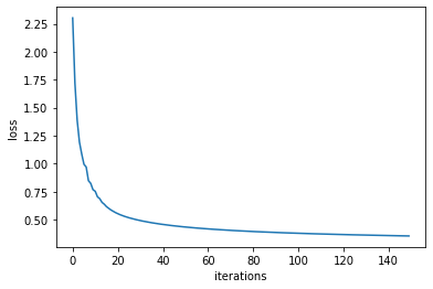
Let us look at the optimization results. Final loss tells us how far we could reduce costs during training process. Further we can use the first loss value as a sanity check and validate our implementation of the loss function works as intended. Recall loss value after first iteration should be approximatly$ -\log(1/c)=\log(c) $ with$ c $ being number of classes. To visulize the whole trainings process we can plot the loss values from each iteration as a loss curve.
# check loss after last iteration
print('last iteration loss:',loss_history[-1])
# Sanity check: first loss should be ln(10)
print('first iteration loss:',loss_history[0])
print('Is the first loss equal to ln(10)?', np.log(10) - loss_history[0] < 0.000001)
# Plot a loss curve
plt.plot(loss_history)
plt.ylabel('loss')
plt.xlabel('iterations')
last iteration loss: 0.35346114237833437
first iteration loss: 2.3025850929940437
Is the first loss equal to ln(10)? True
Evaluation above gave us some inside about the optimization process but did not quantified our final model. One possibility is to calculate model accuracy.
def modelAccuracy(X,y,theta):
    print(X.shape)
    print(y.shape)
    print(theta.shape)
    # calculate probabilities for each digit
    probabilities = softmax(np.dot(X,theta))
    # class with highest probability will be predicted
    prediction = np.argmax(probabilities,axis=1)
    # Sum all correct predictions and divied by number of data
    accuracy = (sum(prediction == np.argmax(y, axis=1)))/X.shape[0]
    return accuracy

print('Training accuracy: ', modelAccuracy(X_train,y_train,opt_theta))
print('Test accuracy: ', modelAccuracy(X_test,y_test,opt_theta))
(60000, 785)
(60000, 10)
(785, 10)
Training accuracy: 0.9027166666666666
(10000, 785)
(10000, 10)
(785, 10)
Test accuracy: 0.9081
Evaluate the Stochastical Gradient Descent Model
# Plot a loss curve
plt.plot(loss_history_sgd)
plt.ylabel('loss')
plt.xlabel('iterations')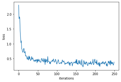
print('Training accuracy: ', modelAccuracy(X_train,y_train,opt_theta_sgd))
print('Test accuracy: ', modelAccuracy(X_test,y_test,opt_theta_sgd))
(60000, 785)
(60000, 10)
(785, 10)
Training accuracy: 0.9069666666666667
(10000, 785)
(10000, 10)
(785, 10)
Test accuracy: 0.9092
Visualize the learnt parameter
One of the benefits of a simple linear model like softmax regression is that we can visualize the parameters$ \theta $ for each of the classes, and see what input it prefers for a strong output.
plt.figure(figsize=(20, 20))
num_classes = 10

for c in range(num_classes):
    f = plt.subplot(10, num_classes, 1 * num_classes + c + 1)
    f.axis('off')
    plt.imshow(np.reshape(opt_theta[1:,c],[28,28]))
plt.show()
Evaluation
Licenses
Notebook License (CC-BY-SA 4.0)
The following license applies to the complete notebook, including code cells. It does however not apply to any referenced external media (e.g., images).
Image Classification - Softmax Regression
by Benjamin Voigt, Klaus Strohmenger, Christian Herta
is licensed under a Creative Commons Attribution-ShareAlike 4.0 International License.
Based on a work at https://gitlab.com/deep.TEACHING.
Code License (MIT)
The following license only applies to code cells of the notebook.
Copyright 2018 Benjamin Voigt, Klaus Strohmenger
Permission is hereby granted, free of charge, to any person obtaining a copy of this software and associated documentation files (the "Software"), to deal in the Software without restriction, including without limitation the rights to use, copy, modify, merge, publish, distribute, sublicense, and/or sell copies of the Software, and to permit persons to whom the Software is furnished to do so, subject to the following conditions:
The above copyright notice and this permission notice shall be included in all copies or substantial portions of the Software.
THE SOFTWARE IS PROVIDED "AS IS", WITHOUT WARRANTY OF ANY KIND, EXPRESS OR IMPLIED, INCLUDING BUT NOT LIMITED TO THE WARRANTIES OF MERCHANTABILITY, FITNESS FOR A PARTICULAR PURPOSE AND NONINFRINGEMENT. IN NO EVENT SHALL THE AUTHORS OR COPYRIGHT HOLDERS BE LIABLE FOR ANY CLAIM, DAMAGES OR OTHER LIABILITY, WHETHER IN AN ACTION OF CONTRACT, TORT OR OTHERWISE, ARISING FROM, OUT OF OR IN CONNECTION WITH THE SOFTWARE OR THE USE OR OTHER DEALINGS IN THE SOFTWARE.