
ML-Fundamentals - Linear Regression - Exercise: Univariate Linear Regression
Table of Contents
Introduction
Linear Regression is the Hello World of Machine Learning. In this exercise you will implement a simple linear regression (univariate linear regression), a model with one predictor and one response variable. The goal is to recap and practice fundamental concepts of Machine Learning. After the exercise, you should have a deeper understanding of what a Machine Learning model is and how do you train such a model with a data set (supervised learning). To achieve this, you will: 1. Calculate the cost and the gradient for concrete training data and$ \theta $ (pen & paper exercise) 2. Create your own data set 3. Implement a linear function as hypothesis (model) 4. Write a function to quantify your model (cost function) 5. Learn to visualize the cost function 6. Implement the gradient descent algorithm to train your model (optimizer) 7. Visualize your training process and results
Requirements
Knowledge
You should have a basic knowledge of Machine Learning models, cost functions, optimization algorithms and also numpy and matplotlib. We will only recap these concepts for a better understanding and do not explain them in great detail. Suitable sources for acquiring this knowledge are:
- Simple Linear Regression Notebook by Christian Herta and his lecture slides (German)
- Chapter 2 of the open classroom Machine Learning by Andrew Ng
- Chapter 5.1 of Deep Learning by Ian Goodfellow
- Some parts of chapter 1 and 3 of Pattern Recognition and Machine Learning by Christopher M. Bishop
- numpy quickstart
- Matplotlib tutorials
Python Modules
By deep.TEACHING convention, all python modules needed to run the notebook are loaded centrally at the beginning.
%matplotlib inline


#%matplotlib notebook
# interactive

# External Modules
import numpy as np
import matplotlib.pyplot as plt
from mpl_toolkits.mplot3d.axes3d import Axes3D
Exercises - Simple Linear Regression
Pen & Paper Exercise
Given the linear model:
$ h_\theta(x) = \theta_0 + \theta_1 x $
And the following concrete training data:
$ D_{train} = \{(0,1),(1,3),(2,6),(4,8)\} $
with each tuple$ (x,y) $ denoting$ x $ the feature and$ y $ the target.
Task:
For$ \theta_0 = 1 $ and$ \theta_1 = 2 $ calculate:
- The cost:
$ J_D(\theta_0, \theta_1)=\frac{1}{2m}\sum_{i=1}^{m}{(h_\theta(x^{(i)})-y^{(i)})^2} $
- The gradient$ \nabla J $, i.e. the partial derivatives:
$ \frac{\partial J (\theta_0, \theta_1)}{\partial \theta_0} $
$ \frac{\partial J (\theta_0, \theta_1)}{\partial \theta_1} $
Create a Data Set
First of all, you have to generate a data set$ \mathcal D_{train} $.$ \mathcal D_{train} $ consists of tuples$ (x^{(i)},y^{(i)}) $. Let$ x $ and$ y $ be two numpy 1d-arrays of equal-length$ m $:
$ {\vec x} = \left(x^{(1)},x^{(2)}, \ldots, x^{(m)}\right)^T \\ {\vec y} = \left(y^{(1)},y^{(2)}, \ldots, y^{(m)}\right)^T $
The$ x $ values should be drawn from a uniform distribution . Add some noise$ \delta $ to the corresponding$ y $ values, which should be drawn from a normal distribution.
$ y^{(i)} = a + b * x^{(i)} + \delta^{(i)} $
We will use an numpy 1d-array for the data which is equivalent to vectors:
\begin{equation} \vec y = a * \vec 1 + b * \vec x + \vec \delta \end{equation}
, with: $ x \sim Uniform([x_{min}, x_{max}]) $ $ \delta \sim Normal(\mu=0.0, \sigma^2=1.0) * n $ $ n $ is an arbitrary nose factor.
An example data set could look like this plot (random seed 42 used):
Hint:
- To generate the vector for$ x $ use the function
np.random.uniform. - To generate a vector of the noise use
np.random.randn.
# fixed random seed
np.random.seed(42)

def linear_random_data(sample_size, a, b, x_min, x_max, noise_factor):
    '''creates a randam data set based on a linear function in a given interval

    Args:
        sample_size: number of data points
        a: coefficent of x^0
        b: coefficent of x^1
        x_min: lower bound value range
        x_max: upper bound value range
        noise_factor: strength of noise added to y

    Returns:
        x: array of x values | len(x)==len(y)
        y: array of y values corresponding to x | len(x)==len(y)
    '''
raise NotImplementedError("You should implement this!")x, y = linear_random_data(sample_size=50, a=0., b=5., x_min=-10, x_max=10, noise_factor=5)
plt.plot(x,y, "rx")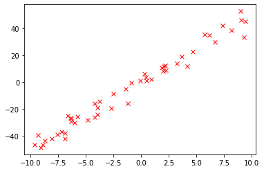
Linear Hypothesis
A short recap, a hypothesis$ h_\theta(x) $ is a certain function that we believe is similar to a target function that we like to model. A hypothesis$ h_\theta(x) $ is a function of$ x $ with fixed parameters$ \theta $. The simplest kind of hypothesis is based on a linear equation with two parameters:
\begin{equation} h_\theta(x) = \theta_{0} + \theta_{1} * x \end{equation}
Implement hypothesis$ h_\theta(x) $ in the method linear_hypothesis and return it as a function.
def linear_hypothesis(theta_0, theta_1):
    ''' Combines given arguments in a linear equation and returns it as a function

    Args:
        theta_0: first coefficient
        theta_1: second coefficient

    Returns:
        lambda that models a linear function based on theta_0, theta_1 and x
    '''
    raise NotImplementedError("You should implement this!")
Cost Function
A cost function$ J $ depends on the given training data$ D $ and hypothesis$ h_\theta(x) $. In the context of the simple linear regression, the cost function measures how wrong a model is regarding its ability to estimate the relationship between$ x $ and$ y $ for specific$ \theta $ values. Later we will treat this as an optimization problem and try to minimize the cost function$ J_D(\theta) $ to find optimal$ \theta $ values for our hypothesis$ h_\theta(x) $. The cost function we use in this exercise is the Mean-Squared-Error (mse) cost function:
\begin{equation} J_D(\theta)=\frac{1}{2m}\sum_{i=1}^{m}{\left(h_\theta(x^{(i)}-y^{(i)})\right)^2} \end{equation}
Implement the cost function$ J_D(\theta) $ in the method mse_cost_function. The method should return a function that takes the values of$ \theta_0 $ and$ \theta_1 $ as an argument.
Sidenote, the terms loss function or error function are often used interchangeably in the field of Machine Learning.
def mse_cost_function(x, y):
    ''' Implements MSE cost function as a function J(theta_0, theta_1) on given tranings data

    Args:
        x: vector of x values
        y: vector of ground truth values y

    Returns:
        lambda J(theta_0, theta_1) that models the cost function
    '''
    raise NotImplementedError("You should implement this!")
j = mse_cost_function(x, y)
print(j(2.1, 2.9))
print(j(2.3, 4.9))88.25403518579944
13.25543063455946
Visualisation of Hypotheses
Now we want to visualize the data set together with the hypothesis and explore the effects of adjusting the parameters. In your plot,
- show your data set as a scatter plot
- show a hypothesis h(x) as a line plot
- calculate and present the MSE cost (a print statement will do as well)
Here are some questions you may want to address:
- How does the line modeling the hypothesis change when you tweak$ \theta_0 $?
- How does the line modeling the hypothesis hypothesis change when you tweak$ \theta_1 $?
- Try some different hypotheses with parameters that are close to the true model and some that are far from the truth. How does this affect the location of the hypothesis in relation to the data?
- What is the effect on the cost?
Your plot could look similar to the following:

def plot_data_with_hypothesis(x, y, theta0, theta1):
    ''' Plots the data (x, y) together with a hypothesis given theta0 and theta1.
    '''
    raise NotImplementedError()
t0 = 0 ### try different values
t1 = 1 ### try different values
plot_data_with_hypothesis(x, y, theta0=t0, theta1=t1)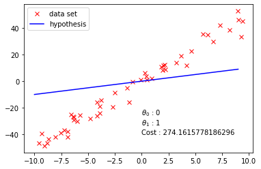
Cost Function Visualization
After implementing a cost function, it is probably a good idea to visualize it to get from an abstract understanding to a more concrete representation. Use matplotlib and plot the cost function in two different ways. Create a contour plot that depicts a three-dimensional surface on a two-dimensional graph and plot the surface itself. Your visualization should consist of two subplots and have corresponding labeling, similar to the following example:

def create_cost_plt_grid(cost, interval, num_samples, theta0_offset=0., theta1_offset=0.):
    '''
    Creates mesh points for a 3D plot based on a given interval and a cost function.
    The function creates a numpy meshgrid for plotting a 3D-plot of the cost function.
    Additionally, for the mesh grid points cost values are calulated and returned.

    Args:
        cost: a function that is used to calculate costs. The function "cost" was typically e.g.
              created by calling "cost = mse_cost_function(x, y)". So, the data x,y and the model
              are used internally in cost. The arguments of the function cost are
              theta_0 und theta_1, i.e. cost(theta_0, theta_0).
        interval: a scalar that defines the range [-interval, interval] of the mesh grid
        num_mesh: the total number of points in the mesh grid is num_mesh * num_mesh (equaly distributed)
        theta0_offset: shifts the plotted interval for theta0 by a scalar
        theta1_offset: shifts the plotted interval for theta1 by a scalar

    Returns:
        T0: a matrix representing a meshgrid for the values of the first plot dimesion (Theta 0)
        T1: a matrix representing a meshgrid for the values of the second plot dimesion (Theta 1)
        C: a matrix respresenting cost values (third plot dimension)
    '''
    raise NotImplementedError("You should implement this!")

def create_cost_plt(T0, T1, Costs):
    ''' Creates a counter and a surface plot based on given data

    Args:
        T0: a matrix representing a meshgrid for X values (Theta 0)
        T1: a matrix representing a meshgrid for Y values (Theta 1)
        C: a matrix respresenting cost values
    '''
    raise NotImplementedError("You should implement this!")
# create some data and plot it
T0, T1, C = create_cost_plt_grid(j, 1000, 51, theta1_offset=5.)
create_cost_plt(T0, T1, C)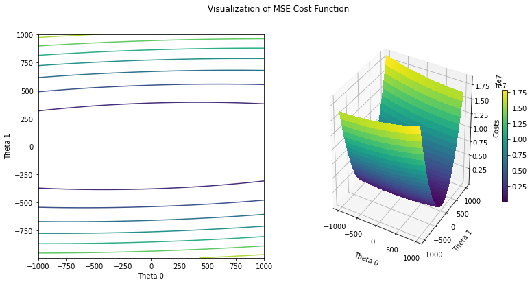
Gradient Descent
A short recap, the gradient descent algorithm is a first-order iterative optimization for finding a minimum of a function. From the current position in a (cost) function, the algorithm steps proportional to the negative of the gradient and repeats this until it reaches a local or global minimum and determines. Stepping proportional means that it does not go entirely in the direction of the negative gradient, but scaled by a fixed value$ \alpha $ also called the learning rate. Implementing the following formalized update rule is the core of the optimization process:
\begin{equation} \theta_{j}^{new} \leftarrow \theta_{j}^{old} - \alpha * \frac{\partial}{\partial\theta_{j}} J(\theta^{old}) \end{equation} $ \frac{\partial}{\partial\theta_{j_{old}}} J(\theta_{old}) $ is the partial derivative (gradient) of the cost function with respect to the j-th parameter.
Partial derivative for$ \theta_0 $: $ \frac{\partial}{\partial \theta_0} J(\Theta) = \frac{1}{m} \sum_{i=1}^m (\theta_0 + \theta_1 \cdot x^{(i)} - y^{(i)}) $
Partial derivative for$ \theta_1 $: $ \frac{\partial}{\partial \theta_1} = \frac{1}{m} \sum_{i=1}^m (\theta_0 + \theta_1 \cdot x^{(i)} - y^{(i)}) \cdot x^{(i)} $
def update_theta(x, y, theta_0, theta_1, learning_rate):
    ''' Updates learnable parameters theta_0 and theta_1

    The update is done by calculating the partial derivities of
    the cost function including the linear hypothesis. The
    gradients scaled by a scalar are subtracted from the given
    theta values.

    Args:
        x: array of x values
        y: array of y values corresponding to x
        theta_0: current theta_0 value
        theta_1: current theta_1 value
        learning_rate: value to scale the negative gradient

    Returns:
        t0: Updated theta_0
        t1: Updated theta_1
    '''
    raise NotImplementedError("You should implement this!")
Using the update_theta method, you can now implement the gradient descent algorithm. Iterate over the update rule to find a$ \theta_0 $ and a$ \theta_1 $ that minimize our cost function$ J_D(\theta) $. This process is often called training of a machine learning model. During the training process create a history of all theta and cost values. You can use them later for evaluation. Implement a verbose argument that if true provides additional information during the process, e.g., final theta values after optimization or cost value at some iterations.
def gradient_descent(x, y, iterations=1000, learning_rate=0.0001, verbose=False):
    ''' Minimize theta values of a linear model based on MSE cost function

    Args:
        x: vector, x values from the data set
        y: vector, y values from the data set
        iterations: scalar, number of theta updates
        learning_rate: scalar, scales the negative gradient
        verbose: boolean, print addition information

    Returns:
        t0s: list of theta_0 values, one value for each iteration
        t1s: list of theta_1 values, one value for each iteration
        costs: list oft costs, one value for each iteration.
    '''
raise NotImplementedError("You should implement this!")cost_hist, t0_hist, t1_hist = gradient_descent(x, y, iterations=250, learning_rate=0.0003, verbose=True)costs: 12.807762911507265
theta_0: 0.74161391410844
theta_1: 4.610072221908946
Model and Training Evaluation
Now visualize the training process by plotting the cost_hist as a curve. Also, create a plot that shows the decision boundary of your final hypothesis (model) inside your data. Your plots should look like:

def evaluation_plt(cost_hist, theta_0, theta_1, x, y):
    ''' Plots a cost curve and the decision boundary

    The Method plots a cost curve from a given training process (cost_hist).
    It also plots the data set (x,y) and draws a linear decision boundary
    with the parameters theta_0 and theta_1 into the plotted data set.

    Args:
        cost_hist: vector, history of all cost values from a opitmization
        theta_0: scalar, model parameter for boundary
        theta_1: scalar, model parameter for boundary
        x: vector, x values from the data set
        y: vector, y values from the data set
    '''
raise NotImplementedError("You should implement this!")evaluation_plt(cost_hist, t0_hist[-1], t1_hist[-1], x, y)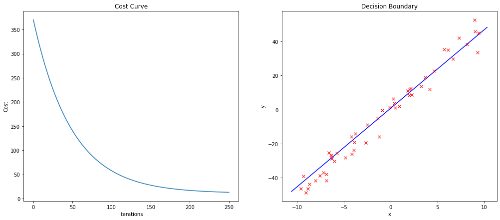
Optimize Hyperparameter
In machine learning, hyperparameters are parameters whose values are set before starting the training process of the model. The learning rate is a hyperparameter, and it is a crucial parameter in the context of optimization with first-order methods in supervised learning. It can easily happen that your model does not learn if you have chosen an unsuited learning rate. To find a suitable learning rate for your problem, you need to try different ones. Implement a function optimize_learning_rate that trains your model with different learning rates and plots the different cost histories. Try to identify edge cases, e.g., cases when the learning rate is too high or too low, to develop a better feeling for the learning rate problem. Your plot could look like this:

def optimize_learning_rate(learning_rates, x, y):
    ''' Train a model with diffrent learning rates and plots the costs

    Args:
        learning_rates: vector, learning rates used to train a linear model
        x: vector, x values from the data set
        y: vector, y values from the data set
    '''
    raise NotImplementedError("You should implement this!")
potential_lr = np.array([0.0001, 0.0007, 0.001, 0.007, .01, .0588, .05899])
optimize_learning_rate(potential_lr, x, y)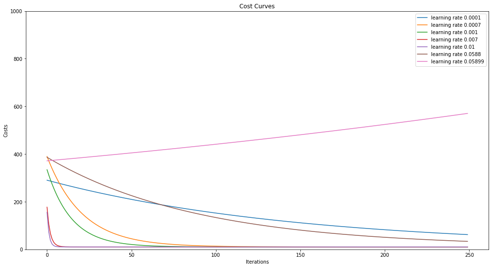
Summary and Outlook
During this exercise, fundamental elements of Machine Learning were covered. You should be able to answer the following questions:
- What is a model using the example of a linear function as a hypothesis?
- How do you quantify a model?
- What is the gradient descent algorithm and what is its used for in the context of Machine Learning?
- Can you explain the concept of hyperparameters and name some?
Licenses
Notebook License (CC-BY-SA 4.0)
The following license applies to the complete notebook, including code cells. It does however not apply to any referenced external media (e.g., images).
Exercise: Simple Linear Regression
by Christian Herta, Benjamin Voigt, Klaus Strohmenger
is licensed under a Creative Commons Attribution-ShareAlike 4.0 International License.
Based on a work at https://gitlab.com/deep.TEACHING.
Code License (MIT)
The following license only applies to code cells of the notebook.
Copyright 2018 Christian Herta, Benjamin Voigt, Klaus Strohmenger
Permission is hereby granted, free of charge, to any person obtaining a copy of this software and associated documentation files (the "Software"), to deal in the Software without restriction, including without limitation the rights to use, copy, modify, merge, publish, distribute, sublicense, and/or sell copies of the Software, and to permit persons to whom the Software is furnished to do so, subject to the following conditions:
The above copyright notice and this permission notice shall be included in all copies or substantial portions of the Software.
THE SOFTWARE IS PROVIDED "AS IS", WITHOUT WARRANTY OF ANY KIND, EXPRESS OR IMPLIED, INCLUDING BUT NOT LIMITED TO THE WARRANTIES OF MERCHANTABILITY, FITNESS FOR A PARTICULAR PURPOSE AND NONINFRINGEMENT. IN NO EVENT SHALL THE AUTHORS OR COPYRIGHT HOLDERS BE LIABLE FOR ANY CLAIM, DAMAGES OR OTHER LIABILITY, WHETHER IN AN ACTION OF CONTRACT, TORT OR OTHERWISE, ARISING FROM, OUT OF OR IN CONNECTION WITH THE SOFTWARE OR THE USE OR OTHER DEALINGS IN THE SOFTWARE.