
Exercises: Variance Reduction by Reparametrization
import numpy as np
from matplotlib import pyplot as plt
from scipy.stats import norm

%matplotlib inline
Introduction
We want to compute the gradient of an expectation:
$ \nabla_\phi \mathbb E_{q_\phi(z)} \left[ f(z) \right] $
Here, we assume that$ f(z) $ has no dependency w.r.t.$ \phi $.
Score Function Estimator
Crude MC estimator
$ \begin{align} \nabla_\phi \mathbb E_{q_\phi(z)} \left[ f(z) \right] &= \mathbb E_{q_\phi(z)} \left[ f(z) \nabla_\phi \log q_\phi(z)\right]\\ & = \int f(z) q_\phi(z) \nabla_\phi \log q_\phi(z) dz \\ \end{align} $
The integral can be estimated by Monte-Carlo with sampling of the hidden variables$ z^{(i)} $ from$ q_\phi(z) $ (notation:$ z^{(i)}\sim q_\phi(z) $):
$ \int f(z) q_\phi(z) \nabla_\phi \log q_\phi(z) dz \approx \frac{1}{n} \sum_{i=1}^n f(z^{(i)})\nabla_\phi \log q_\phi(z^{(i)}) $
The problem of the crude MC estimator is that it has high variance.
Example
Let's keep the things simple. We use a Gaussian for our distribution$ q_{\phi}(z^{(i)}) $ with$ \phi = \{ \mu, \sigma^2\} $:
$ \mathcal N (z \mid \mu, \sigma^2) = \frac{1}{\sqrt{2\pi \sigma^2}} \exp(-\frac{(z-\mu)^2}{2 \sigma^2}) $
As function we use$ f(z)=z^2 $.
loc=mu=10.
scale=3.
sigma2 = scale**2
size=100

def sample_z_from_q(loc=loc, scale=scale, size=size):
    return np.random.normal(loc=loc, scale=scale, size=size)
def f(z):
return z**2Show that the derivatives w.r.t.$ \mu $ and$ \sigma^2 $ are:
$ \frac{\partial}{\partial \mu} \log \mathcal N (z \mid \mu, \sigma^2) = \frac{(z-\mu)}{\sigma^2}\\ $
$ \frac{\partial}{\partial \sigma^2} \log \mathcal N (z \mid \mu, \sigma^2) = - \frac{1}{2 \sigma^2}+ \frac{(z-\mu)^2}{2 (\sigma^2)^2}\\ $
$ \begin{align} \frac{\partial}{\partial \mu} \log \mathcal N (z \mid \mu, \sigma^2) &= \frac{\partial}{\partial \mu} \log \left(\frac{1}{\sqrt{2\pi \sigma^2}} \exp(-\frac{(z-\mu)^2}{2 \sigma^2})\right)\\ &= \frac{\partial}{\partial \mu} \left(\log \left(\frac{1}{\sqrt{2\pi \sigma^2}} \right)+ \left(\log \exp(-\frac{(z-\mu)^2}{2 \sigma^2})\right)\right)\\ &= \frac{\partial}{\partial \mu} \log \left(\frac{1}{\sqrt{2\pi \sigma^2}} \right)+ \frac{\partial}{\partial \mu} \left(\log \exp(-\frac{(z-\mu)^2}{2 \sigma^2})\right)\\ &= 0 - \frac{\partial}{\partial \mu}\frac{(z-\mu)^2}{2 \sigma^2}\\ &= \frac{(z-\mu)}{\sigma^2}\\ \end{align} $
$ \begin{align} \frac{\partial}{\partial \sigma^2} \log \mathcal N (z \mid \mu, \sigma^2) &= \frac{\partial}{\partial \sigma^2} \log \left(\frac{1}{\sqrt{2\pi \sigma^2}} \exp(-\frac{(z-\mu)^2}{2\sigma^2})\right) \\ &= \frac{\partial}{\partial \sigma^2} \left(\log \left(\frac{1}{\sqrt{2\pi \sigma^2}} \right)+ \left(\log \exp(-\frac{(z-\mu)^2}{2\sigma^2})\right)\right)\\ &= \frac{\partial}{\partial \sigma^2} \log \left(\frac{1}{\sqrt{2\pi \sigma^2}} \right)+ \frac{\partial}{\partial \sigma^2} \left(\log \exp(-\frac{(z-\mu)^2}{2\sigma^2})\right)\\ &= - \frac{\partial}{\partial \sigma^2} \log \left(\sqrt{2\pi \sigma^2} \right)+ \frac{\partial}{\partial \sigma^2} \left(\log \exp(-\frac{(z-\mu)^2}{2 \sigma^2})\right)\\ &= - \frac{1}{2 \sigma^2}+ \frac{(z-\mu)^2}{2 (\sigma^2)^2}\\ \end{align} $
def dq_dmu(z, mu=mu, sigma2=sigma2):
    return (z - mu)/sigma2

def dq_dsigma2(z, mu=mu, sigma2=sigma2):
    return - 1/(2*sigma2) + (z-mu)**2/sigma2**2
Exercise: Implement the Crude MC estimator:
$ \begin{align} \frac{\partial}{\partial \mu} \mathbb E_{\mathcal N (z \mid \mu, \sigma^2) } \left[ f(z) \right] &= \mathbb E_{\mathcal N (z \mid \mu, \sigma^2) } \left[ f(z) \frac{\partial}{\partial \mu} \log \mathcal N (z \mid \mu, \sigma^2)\right]\\ & \approx \frac{1}{n} \sum_{i=1}^n f(z^{(i)}) \frac{\partial}{\partial \mu} \log \mathcal N (z \mid \mu, \sigma^2) = \frac{1}{n} \sum_{i=1}^n f(z^{(i)}) \frac{(z^{(i)}-\mu)}{\sigma^2} \end{align} $
def get_crude_mc_estimates(size):
    estimates = []
    for i in range(10000):
        estimate = crude_mc_estimate(size=size, f=f, dq_dmu=dq_dmu)
        estimates.append(estimate)
    return np.array(estimates)
estimates = get_crude_mc_estimates(size=100)
plt.hist(estimates);
#plt.xlim(15, 25)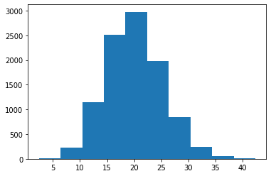
estimates = get_crude_mc_estimates(size=10000)
plt.hist(estimates);
plt.xlim(15, 25)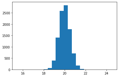
Reparametrization for variance reduction
$ z = g_\phi(\epsilon) $
$ \nabla_\phi \mathbb E_{q_\phi(z)} \left[ f(z) \right] = \mathbb E_{p(\epsilon)} [\nabla_\phi f (g_\phi(\epsilon))] $ $ p(\epsilon) $ is a (fixed) distribution with no dependence on$ \phi $.
Here: -$ p(\epsilon) = \mathcal N(0, 1) $ -$ g_{\mu, \sigma^2}(\epsilon) = \mu + \epsilon \sigma $
Exercise
- Implement the reparametrized MC estimator
$ \frac{\partial}{\partial \mu} \mathbb E_{\mathcal N (z \mid \mu, \sigma^2) } \left[ f(z) \right] = \mathbb E_{p(\epsilon)} \left[\frac{\partial}{\partial \mu} f (g_{\mu, \sigma^2}(\epsilon))\right] $
- Find a mathematical expression for$ \frac{\partial f}{\partial \mu} $ and use it in the estimator.
- Sample$ \epsilon \sim \mathcal N(0, 1) $
def sample_epsilon_from_p(size=size): # no dependence on mu and sigma2
    return np.random.normal(loc=0, scale=1, size=size)
$ \nabla_\phi f (g_\phi(\epsilon)) $
$ g = \mu + \epsilon \sigma $
$ z = g_{\mu, \sigma^2}(\epsilon) $
$ f(z) = f(g) = g^2 $
$ \frac{\partial f}{\partial \mu} = \frac{\partial f}{\partial g}\frac{\partial g}{\partial \mu} = 2 g $
def get_reparametrized_mc_estimates(size):
    estimates = []
    for i in range(10000):
        estimate= reparametrized_mc_estimate(size)
        estimates.append(estimate)
    return np.array(estimates)
def g(epsilon, mu=mu, sigma2=sigma2):
return mu + epsilon * np.sqrt(sigma2)def reparametrized_mc_estimate(size):
epsilons = sample_epsilon_from_p(size)
return (2 * g(epsilons)).mean()# here we need just 100 samples to get a similar result as for 10000 "crude" mc samples
estimates = get_reparametrized_mc_estimates(100)
plt.hist(estimates);
plt.xlim(15, 25)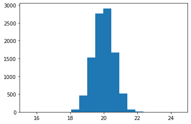
#### for 10000 samples
estimates = get_reparametrized_mc_estimates(10000)
plt.hist(estimates);
plt.xlim(15, 25)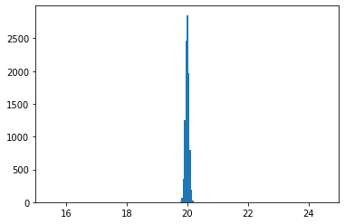
Comparision between crude MC and reparametrized MC
crude_mc_var = []
reparam_mc_var = []
ns = np.array([10,30,90,300,600,900, 1500, 3000])
for i in ns:
    crude_mc_estimates = get_crude_mc_estimates(size=i)
    reparam_mc_estimates = get_reparametrized_mc_estimates(size=i)
    crude_mc_var.append(crude_mc_estimates.var(ddof=1))
    reparam_mc_var.append(reparam_mc_estimates.var(ddof=1))
crude_mc_var = np.array(crude_mc_var)
reparam_mc_var = np.array(reparam_mc_var)plt.figure(figsize=(10, 8))
plt.loglog(ns, crude_mc_var, "bo", label="crude mc")
plt.loglog(ns, crude_mc_var, "b-")
plt.loglog(ns, reparam_mc_var, "go", label="reparametrized mc")
plt.loglog(ns, reparam_mc_var, "g-")
plt.xlabel("number of samples")
plt.ylabel("(empirical) variance of the estimators")
plt.legend();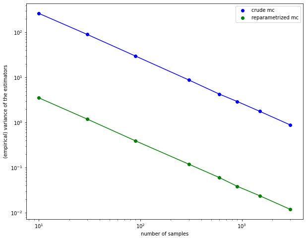
As you can see from the plot there is a strait line in a log-log plot:
$ \log y = a + b \log x $
therefore (with$ c = \exp(a) $): $ y = c x^b $
We know:
$ var(estimate) = \frac{c}{n} $
so be must be$ -1 $. Let's check this:
b_crude = (np.log(crude_mc_var[-1]) - np.log(crude_mc_var[0]))/(np.log(ns[-1])-np.log(ns[0]))
b_crude
b_reparm = (np.log(reparam_mc_var[-1]) - np.log(reparam_mc_var[0]))/(np.log(ns[-1])-np.log(ns[0]))
b_reparm$ a = \log y - b \log x $
# with b \approx 1
as_reparam = np.log(reparam_mc_var) + np.log(ns)
cs_reparam = np.exp(as_reparam)
cs_reparam.mean()
# with b \approx 1
as_crude = np.log(crude_mc_var) + np.log(ns)
cs_crude= np.exp(as_crude)
cs_crude.mean()$ var(estimate\_reparam) = \frac{35.8}{n} $
$ var(estimate\_crude) = \frac{2648}{n} $
$ \eta_{VR} =\frac{\text{var}\left(\hat H_n\right)-\text{var}\left(\bar H_n\right)}{\text{var}\left(\hat H_n\right)} $
eta = (2648-35.8)/2648
eta
# Here we need approx. 1.35% of the samples to get the same
# variance with our variance reduction technique
35.8/2648Literature
- Diederik P. Kingma, Max Welling: Auto-Encoding Variational Bayes,
- Diederik P. Kingma, Max Welling: Efficient Gradient-based Inference through Transformation between Bayes Nets and Neural Nets,