
Exercise - Estimating Mean and Standard Deviation of Normal Distribution with Pyro
Table of Contents
Introduction
"Pyro is a universal probabilistic programming language (PPL) written in Python and supported by PyTorch on the backend. Pyro enables flexible and expressive deep probabilistic modeling, unifying the best of modern deep learning and Bayesian modeling." (https://pyro.ai/).
In this exercise you will use Pyro to estimate the parameters of a normal distribution.
In order to detect errors in your own code, execute the notebook cells containing assert or assert_almost_equal.
Requirements
Knowledge
Theory
All Pyro-exercises are intended as part of the course Bayesian Learning. Therefore work through the course up to and including chapter Probabilistic Programming.
Pyro
Python Modules
import numpy as np

import scipy.stats
from scipy.stats import norm

from matplotlib import pyplot as plt
from IPython.core.pylabtools import figsize

%matplotlib inline
import torch
from torch.distributions import constraints
import pyro
import pyro.infer
import pyro.optim as optim
import pyro.distributions as distData
Our observed data comes from a normal distribution:
Data: $ X \sim \mathcal N(\mu, \frac{1}{\tau}) $
Probability Density Function: $ p(X \mid \mu, \tau) = \sqrt{\frac{\tau}{2\pi}} \exp\left( -\frac{\tau (X-\mu)^2 }{2} \right) $
with
-$ \mu $: mean
-$ \sigma^2 $: variance
-$ \tau =\frac{1}{\sigma^2} $ : precision
dtype=torch.float32torch.manual_seed(101)
pyro.set_rng_seed(101)
np.random.seed(12);# generate observed data
N = 10
mu_ = 10.
sigma_= 2.
X = np.random.normal(mu_, sigma_, N)
X = np.array(X, dtype=np.float32)Xx = np.arange(3,18,0.01)
p_x = scipy.stats.norm.pdf(x, loc=mu_, scale=sigma_)
plt.plot(x, p_x, label="true distribution")
plt.plot(X, np.zeros_like(X), "ro", label="observed data")
plt.title("")
plt.xlabel("x")
plt.ylabel("p(x)")
plt.legend();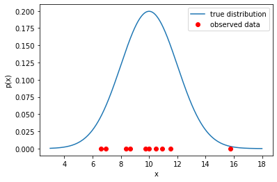
Working with Pyro
The Model
We use the generated data$ X \sim \mathcal N(\mu, 1/\tau) $ as observed data.
For modeling the data we design the following model with pyro:
- We use a Uniform prior for the mean$ \mu $: *$ \mu \sim \text{Uniform}(-25,25) $
-
We use a constant$ \tau=1/4 $ for the precision.
-
Note: This has to be a
torch.tensorobject
-
So, we have only one (scalar) parameter$ \theta=\{\mu\} $ in the model.
def model(X):
    # Prior
    mu = pyro.sample("mu", dist.Uniform(torch.tensor(-25.), torch.tensor(+25.)))
    tau = torch.tensor(1/4)


    # pyro plate mark the samples as conditional independet
    with pyro.plate("observed_data", size=len(X)):
        sample = pyro.sample("gaussian_data", dist.Normal(mu, 1/torch.sqrt(tau)), obs=X)

    return sample
The Guide
Next we implement the "Guide", which we will later on use in conjuction with our model for stochastic variational inference (pyro.infer.SVI()).
We use as variational distribution also a Gaussian. $ \mu \sim \mathcal N(mean_{\mu}, scale_{\mu}^2) $
### same (function) arguments for guide and model !
def guide(X):
    mean_loc = torch.randn((1))
    # note that we initialize the scale to be pretty narrow
    mean_scale = torch.tensor(0.001)

    # mu_loc and mu_scale are the (variational) parameters
    # they will be learned by SVI from the data

    mu_loc = pyro.param("guide_mu_mean", mean_loc)

    # the scale must be positive.
    mu_scale = pyro.param("guide_mu_scale", mean_scale, constraint=constraints.positive)

    # note the same name "mu" here as in our model
    mu = pyro.sample("mu", dist.Normal(mu_loc, mu_scale))
Stochastic Variational Inference - SVI
Now we optimize the variational parameters, i.e. find values for$ mean_{\mu} $(guide_mu_loc) ,$ scale_{\mu} $(guide_mu_scale).
pyro.clear_param_store()

adam_params = {"lr": 0.003, "betas": (0.95, 0.999)}
optimizer = optim.Adam(adam_params)

svi = pyro.infer.SVI(model=model,
                     guide=guide,
                     optim=optimizer,
                     loss=pyro.infer.Trace_ELBO())
### to keep track of our loss history
losses = []
### convert observed data to a torch tensor object
X_ = torch.tensor(X, dtype=dtype)
### training / inference
for t in range(10000):
### svi.step takes same parameters as inpust as our defined model(X) and guide(X) function
loss = svi.step(X_)
losses.append(loss)
### for monitoring
if t%100==0:
print (t, "\t", loss)0 192.7898645401001
100 182.77566051483154
200 175.62650108337402
300 167.52554512023926
400 160.4677028656006
500 152.7523307800293
600 145.86118698120117
700 138.8842272758484
800 132.40819215774536
900 125.13015508651733
1000 120.28953409194946
1100 114.50648021697998
1200 109.0264321565628
1300 104.05447161197662
1400 98.44436323642731
1500 94.8081842660904
1600 88.7485808134079
1700 82.15620362758636
1800 81.87902522087097
1900 79.11943554878235
2000 75.53384268283844
2100 66.19532096385956
2200 68.04433608055115
2300 66.57482993602753
2400 62.50554394721985
2500 58.092737913131714
2600 50.86673945188522
2700 50.28860080242157
2800 50.554264426231384
2900 51.21060395240784
3000 52.01752185821533
3100 46.69825541973114
3200 46.012785851955414
3300 36.88210213184357
3400 39.41662901639938
3500 38.12995171546936
3600 37.32512640953064
3700 36.20981675386429
3800 27.626056909561157
3900 33.031264930963516
4000 36.130385994911194
4100 30.761741161346436
4200 33.44706857204437
4300 32.17227989435196
4400 27.44186782836914
4500 28.889544129371643
4600 28.15209126472473
4700 27.93236869573593
4800 32.44645023345947
4900 26.777266144752502
5000 26.466034293174744
5100 28.466201186180115
5200 29.26971936225891
5300 28.370587825775146
5400 27.29229199886322
5500 28.670193433761597
5600 27.79488968849182
5700 26.52428138256073
5800 27.6370712518692
5900 26.795197248458862
6000 27.617044389247894
6100 27.531768143177032
6200 27.32448798418045
6300 27.33493372797966
6400 27.09856367111206
6500 27.16217875480652
6600 27.344936847686768
6700 27.19107562303543
6800 27.275490045547485
6900 27.227381706237793
7000 27.38326871395111
7100 27.271712124347687
7200 27.275525629520416
7300 27.29395294189453
7400 27.296905517578125
7500 27.358410716056824
7600 27.299220591783524
7700 27.37580680847168
7800 27.317962676286697
7900 27.308402448892593
8000 27.23542332649231
8100 27.245432496070862
8200 27.318854212760925
8300 27.30628141760826
8400 27.346500039100647
8500 27.337133824825287
8600 27.397686779499054
8700 27.34884524345398
8800 26.45894765853882
8900 27.251322388648987
9000 27.27135920524597
9100 27.359524488449097
9200 27.374260008335114
9300 27.31026601791382
9400 27.368039429187775
9500 27.321097254753113
9600 27.248512744903564
9700 27.3205828666687
9800 27.32727861404419
9900 27.327588766813278
### Let us plot the costs / iteration curve

plt.xlabel("# iteration")
plt.ylabel("MC-Estimate of ELBO")
plt.plot(range(len(losses)), losses)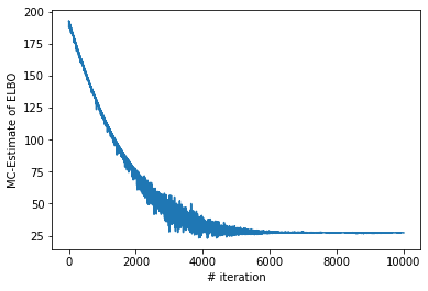
# Adjust the strings according to your names for
# the parameters "mu_mean", etc...
mu_mean_param = pyro.param("guide_mu_mean")
mu_scale_param = pyro.param("guide_mu_scale")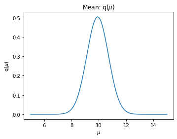
mu_mean_param, mu_scale_paramplt.figure(figsize=(12,4))
mu_mean = mu_mean_param.detach().numpy()
mu_scale = mu_scale_param.detach().numpy()
x = np.arange(5,15,0.01)
p_mu = scipy.stats.norm.pdf(x, loc=mu_mean, scale=np.sqrt(mu_scale))
ax = plt.subplot(121)
ax.plot(x, p_mu)
ax.set_xlabel("$\mu$")
ax.set_ylabel("q($\mu$)")
ax.set_title("Mean: q($\\mu$)")
print("true mu: ", mu_)true mu: 10.0
Exercise - Estimate Precision and Mean
Task:
Extend the model and the guide by using additionally a variational distribution for$ \tau $:
- Use a Uniform distribution for the proir of$ \tau $:$ \tau \sim \text{Uniform}(0.01, 2) $
- Use a Gamma distribution as variational distribution for$ \tau $:$ \text{Gamma}(a, b) $
- Additionally, find the parameters$ a $ (
guide_tau_concentration),$ b $ (guide_tau_rate) (and$ mean_{\mu} $guide_mu_mean,$ scale_{\mu} $guide_mu_scale) via optimization.
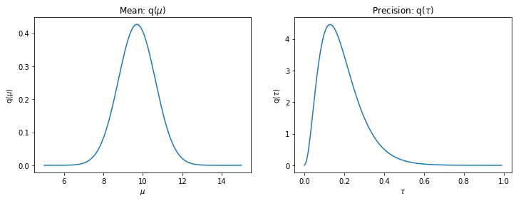
If your extensions are correct, executing the cells at the end should plot figures similar to these:
Gamma Function
Use the plot of a gamma function to find appropriate values for the variational parameters.
concentration = 1.5
rate = 1.

x = np.arange(0,4,0.01)
p_tau = scipy.stats.gamma.pdf(x, a=concentration, scale=1/rate)
plt.xlabel("x")
plt.ylabel("p(x)")
plt.plot(x, p_tau)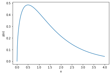
# Note that dist.Gamma has a different parameter signature: __init__(self, concentration, rate, validate_args=None)
# see:
#help(dist.Gamma)
def model_with_tau(X):
######################
### Your Code here ###
######################
returndef guide_with_tau(X):
######################
### Your Code here ###
######################
return### Initilize pyro.infer.SVI object
######################
### Your Code here ###
######################### Training
######################
### Your Code here ###
######################### Let us plot the costs / iteration curve
plt.xlabel("# iteration")
plt.ylabel("MC-Estimate of ELBO")
plt.plot(range(len(losses)), losses)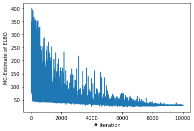
# Adjust the strings according to your names for
# the parameters "mu_mean", etc...
mu_mean_param = pyro.param("guide_mu_mean")
mu_scale_param = pyro.param("guide_mu_scale")
mu_mean_param, mu_scale_param
# Adjust the strings according to your names for
# the parameters "mu_mean", etc...
tau_concentration_param = pyro.param("guide_tau_concentration")
tau_rate_param = pyro.param("guide_tau_rate")
tau_concentration_param, tau_rate_paramplt.figure(figsize=(12,4))
mu_mean = mu_mean_param.detach().numpy()
mu_scale = mu_scale_param.detach().numpy()
x = np.arange(5,15,0.01)
p_mu = scipy.stats.norm.pdf(x, loc=mu_mean, scale=np.sqrt(mu_scale))
ax = plt.subplot(121)
ax.plot(x, p_mu)
ax.set_xlabel("$\mu$")
ax.set_ylabel("q($\mu$)")
ax.set_title("Mean: q($\\mu$)")
print("true mu: ", mu_)
tau_concentration =tau_concentration_param.detach().numpy()
tau_rate = tau_rate_param.detach().numpy()
x = np.arange(0,1,0.01)
p_tau = scipy.stats.gamma.pdf(x, a=tau_concentration, scale=1/tau_rate)
ax = plt.subplot(122)
ax.plot(x, p_tau)
ax.set_xlabel("$\\tau$")
ax.set_ylabel("q($\\tau$)")
ax.set_title("Precision: q($\\tau$)")
print("true tau: ", 1/sigma_**2)
true mu:  10.0
true tau:  0.25
Licenses
Notebook License (CC-BY-SA 4.0)
The following license applies to the complete notebook, including code cells. It does however not apply to any referenced external media (e.g., images).
Exercise - Pyro Simple Gaussian
by Christian Herta
is licensed under a Creative Commons Attribution-ShareAlike 4.0 International License.
Based on a work at https://gitlab.com/deep.TEACHING.
Code License (MIT)
The following license only applies to code cells of the notebook.
Copyright 2019 Christian Herta
Permission is hereby granted, free of charge, to any person obtaining a copy of this software and associated documentation files (the "Software"), to deal in the Software without restriction, including without limitation the rights to use, copy, modify, merge, publish, distribute, sublicense, and/or sell copies of the Software, and to permit persons to whom the Software is furnished to do so, subject to the following conditions:
The above copyright notice and this permission notice shall be included in all copies or substantial portions of the Software.
THE SOFTWARE IS PROVIDED "AS IS", WITHOUT WARRANTY OF ANY KIND, EXPRESS OR IMPLIED, INCLUDING BUT NOT LIMITED TO THE WARRANTIES OF MERCHANTABILITY, FITNESS FOR A PARTICULAR PURPOSE AND NONINFRINGEMENT. IN NO EVENT SHALL THE AUTHORS OR COPYRIGHT HOLDERS BE LIABLE FOR ANY CLAIM, DAMAGES OR OTHER LIABILITY, WHETHER IN AN ACTION OF CONTRACT, TORT OR OTHERWISE, ARISING FROM, OUT OF OR IN CONNECTION WITH THE SOFTWARE OR THE USE OR OTHER DEALINGS IN THE SOFTWARE.