import numpy as np
# for a gpu version 
# import cupy as np

from matplotlib import pyplot as plt
%matplotlib inline

# we use the lightweight deep learning library dp
# you have to put dp.py in the same folder as this noebook
# you can download it from
# https://gitlab.com/deep.TEACHING/educational-materials/-/blob/master/notebooks/differentiable-programming/dp.py
# if you have downloaded the complete deep teaching git repo you find it in the folder ../differentiable-programming/

import dp # differentiable programming module
from dp import Node

#data_path = "/Users/christian/data/mnist_csv/"
data_path = "/home/chris/Downloads/"
# get the data from
#   https://pjreddie.com/projects/mnist-in-csv/

try:
    train_data_mnist
except NameError:
    train_data_mnist = np.loadtxt(data_path + "mnist_train.csv", delimiter=",")
    test_data_mnist = np.loadtxt(data_path + "mnist_test.csv", delimiter=",")

original_dim = 784 # Number of pixels in MNIST images.
latent_dim = 5 # dimensionality of the latent code z.
intermediate_dim = 128 # Size of the hidden layer.
epochs = 30
image_dim = int(np.sqrt(original_dim))
image_dim

def get_xy_mnist(data_mnist=train_data_mnist):
    x_train = train_data_mnist[:,1:]
    x_train = x_train / 255. 
    #x_train = x_train.reshape((-1, image_dim, image_dim))
    y_train = train_data_mnist[:,0]
    return x_train, y_train

x_train_, y_train_ = get_xy_mnist()
x_test_, y_test = get_xy_mnist(test_data_mnist)

nb_classes = 10
m = y_train_.shape[0]
y_train = np.zeros((m, nb_classes), dtype=int)
y_train[np.arange(m), y_train_.astype(int)] = 1

batch_size = 2**7
batch_size

def random_batch(x_train=x_train, y_train=y_train, batch_size=batch_size):
    n = x_train.shape[0]
    indices = np.random.randint(0,n, size=batch_size)
    return x_train[indices], y_train[indices]

class VAE(dp.Model):
    
    def __init__(self, original_dim=original_dim, 
                 intermediate_dim=intermediate_dim, 
                 latent_dim=latent_dim):
        super(VAE, self).__init__()
        
        # encoder param
        self.fc1 = self.ReLu_Layer(original_dim, intermediate_dim, "fc1")
        self.fc21 = self.Linear_Layer(intermediate_dim, latent_dim, "fc21")
        self.fc22 = self.Linear_Layer(intermediate_dim, latent_dim, "fc22")
        
        # decoder param
        self.fc3 = self.ReLu_Layer(latent_dim, intermediate_dim, "fc3")
        self.fc4 = self.Linear_Layer(intermediate_dim, original_dim, "fc4")
    
    def encoder(self, x):
        h1 = self.fc1(x)
        return self.fc21(h1), self.fc22(h1)
    
    def decoder(self, z):
        h3 = self.fc3(z)
        return self.fc4(h3).sigmoid()

    # Sampling from the distribution q(z | x) = N(loc, scale)
    # with reparametrization trick.
    def sampling(mu, logvar):
        # as exercise
        raise NotImplementedError()
    
    def elbo_binomial(x, x_decoded_mean, z_mean, z_logvar):
        # as exercise
        raise NotImplementedError()
        
    def complete_result(self, x, y=None):
        assert isinstance(x, Node)
        x_reconstructed, z, mu, logvar = self.encoder_decoder(x)
        loss = VAE.elbo_binomial(x, x_reconstructed, mu, logvar)
        return loss, x_reconstructed, z, mu, logvar
             
    def loss(self, x, y=None):
        loss, x_reconstructed, z, mu, logvar = self.complete_result(x)
        return loss
        
    def encoder_decoder(self, x=None): 
        assert isinstance(x, Node)
        mu, logvar = self.encoder(x)
        z = VAE.sampling(mu, logvar)
        x_reconstructed = self.decoder(z)
        return x_reconstructed, z, mu, logvar 
    

model = VAE()

optimizer = dp.optimizer.RMS_Prop(model, x_train, y_train, {"alpha":0.001, "beta2":0.9}, batch_size=batch_size)
optimizer.train(steps=2000, print_each=100)

# TODO: new image plots!

b_size = 10
x_, y_ = random_batch(batch_size=b_size)
x_1, y_1 = random_batch(x_test, y_test, batch_size=b_size)

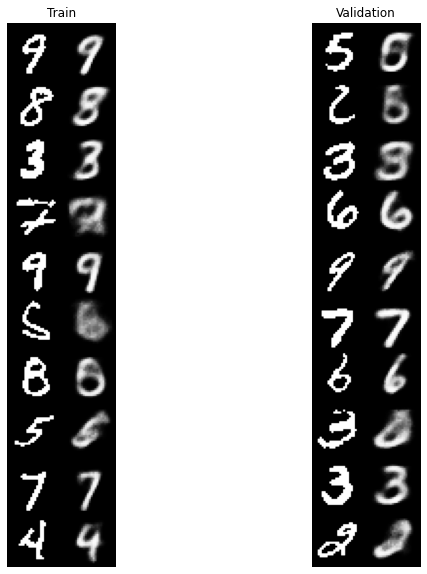
fig = plt.figure(figsize=(10, 10))
for fid_idx, (data, title) in enumerate(
            zip([x_, x_1], ['Train', 'Validation'])):
    n = 10  # figure with 10 x 2 digits
    digit_size = image_dim
    figure = np.zeros((digit_size * n, digit_size * 2))
    
    loss, x_reconstructed, z, mu, logvar = model.complete_result(x=Node(data))
    decoded = x_reconstructed.value
    decoded = np.clip(decoded,0,1)
    for i in range(10):
        figure[i * digit_size: (i + 1) * digit_size,
               :digit_size] = data[i, :].reshape(digit_size, digit_size)
        figure[i * digit_size: (i + 1) * digit_size,
               digit_size:] = decoded[i, :].reshape(digit_size, digit_size)
    ax = fig.add_subplot(1, 2, fid_idx + 1)
    ax.imshow(figure, cmap='Greys_r')
    ax.set_title(title)
    ax.axis('off')
plt.show()

n_samples = 10
# Todo as exercise
sampled_im_mean = None # Todo as exercise

# TODO: new image plots!
# Show the sampled images.
plt.figure()
for i in range(n_samples):
    ax = plt.subplot(n_samples // 5 + 1, 5, i + 1)
    plt.imshow(sampled_im_mean[i, :].reshape(28, 28), cmap='gray')
    ax.axis('off')
plt.show()

# VAE conditioned on class label
class Conditional_VAE(dp.Model):
    def __init__(self, original_dim=original_dim, 
                 intermediate_dim=intermediate_dim, 
                 latent_dim=latent_dim,
                 nb_classes=nb_classes
                ):
        super(Conditional_VAE, self).__init__()
        
        # encoder param
        self.fc1 = self.ReLu_Layer(original_dim+nb_classes, intermediate_dim, "fc1")
        self.fc21 = self.Linear_Layer(intermediate_dim, latent_dim, "fc21")
        self.fc22 = self.Linear_Layer(intermediate_dim, latent_dim, "fc22")
        
        # decoder param
        self.fc3 = self.ReLu_Layer(latent_dim+nb_classes, intermediate_dim, "fc3")
        self.fc4 = self.Linear_Layer(intermediate_dim, original_dim, "fc4")
    
    def encoder(self, x, y):
        xy = x.concatenate(y, axis=1)
        h1 = self.fc1(xy)
        return self.fc21(h1), self.fc22(h1)
    
    def decoder(self, z, y):
        zy = z.concatenate(y, axis=1)
        h3 = self.fc3(zy)
        return self.fc4(h3).sigmoid()

    def complete_result(self, x, y):
        assert isinstance(x, Node)
        x_reconstructed, z, mu, logvar = self.encoder_decoder(x, y)
        loss = VAE.elbo_binomial(x, x_reconstructed, mu, logvar)
        return loss, x_reconstructed, z, mu, logvar
             
    def loss(self, x, y):
        loss, x_reconstructed, z, mu, logvar = self.complete_result(x, y)
        return loss
        
    def encoder_decoder(self, x, y): 
        assert isinstance(x, Node)
        assert isinstance(y, Node)
        mu, logvar = self.encoder(x, y)
        z = VAE.sampling(mu, logvar)
        x_reconstructed = self.decoder(z, y)
        return x_reconstructed, z, mu, logvar 

cmodel = Conditional_VAE()

optimizer = dp.optimizer.RMS_Prop(cmodel, x_train, y_train, 
                                  {"alpha":0.001, "beta2":0.9}, batch_size=batch_size)
optimizer.train(steps=3000, print_each=100)

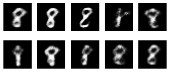
# sampled_image_mean has size 10 x 784 with 10
nb_samples = 10
z = np.random.normal(size=(n_samples, latent_dim))

# Ths is the number which is generated as image
label = 8


y = np.zeros([nb_samples, nb_classes])
y[:, label] = 3.
sampled_im_mean = cmodel.decoder(Node(z), Node(y)).value

# TODO: new image plots!
# Show the sampled images.
plt.figure()
for i in range(n_samples):
    ax = plt.subplot(n_samples // 5 + 1, 5, i + 1)
    plt.imshow(sampled_im_mean[i, :].reshape(28, 28), cmap='gray')
    ax.axis('off')
plt.show()