
Status: Draft
Introduction to Machine Learning
In order to really understand how neural networks work, it is essential to understand their core concepts. Practically, a multi layer perceptron (fully connected feed forward network) consists of many logistic regression tasks. So in order to understand neural networks you need to understand logistic regression, which is practically linear regression extended with a sigmoid function.
Linear regression is used to predict continous values (e.g. the temperature tomorrow), based on some features (e.g. temperature today, humidity, calender week, etc…). By adding a sigmoid function at the end of linear regression, the final output will be a value between 0.0 and 1.0. Adding a threshold at 0.5 then results in a binary classifier (e.g. warm or cold day tomorrow).
Stacking several logistic regressions (though with other activation function) in the same layer after the input layer and adding a last logistic regression after that, results in a fully connected neural network with one hidden layer. But this will be tought in the next course Introduction to Neural Networks
Exercises
The following exercises are meant to be done in chronological order as listes below. There are versions using Python-numpy only and versions, which make use of the deep learning framework PyTorch. For the best learning effect, we suggest to do all numpy exercises first and then proceed with the PyTorch exercises.
Prerequisites
Math
Training and using regression models, and therefore also neural networks, requires either a lot of loops (seriously, do not use loops!), or better, matrix and vector operations. The first exercise is intended to refresh mathematic skills.
Scientific Python
In Python, the most efficient way to handle vectors, matrices and n-dimensional arrays is via the package numpy. Its core functions are implemented in C and Fortran, which makes it extremely fast. Numpy provides a lot of functions and features to access and manipulate n-dimensional arrays. Having a basic knowledge about what is possible with numpy will ease any data-scientists daily work with Python. Therefore we strongly suggest going through this course first:
Regression
The most simple model to start with is linear regression. In the regression exercises you will build a model, which predicts a floating point value (target value), based on only one or more other floating point values (features). You will get familiar with the concept of hypotheses, cost functions (here mean squared error), the gradient descent algorithm and the iterative update rule.
Univariate Linear Regression
Imagine you want to predict the house price (target value $y$), based sololy on one feature $x$, e.g. the area in sqm. You get some example data $D_{Train} = \{(x^{(1)}, y^{(1)}), (x^{(2)}, y^{(2)}), \ldots, (x^{(m)}, y^{(m)})\}$, which consists of pairs of $(x^{(i)}, y^{(i)})$. Unfortunately, the data does not contain any example, which has exactly the sqm you want to know the price for. The most simple thing to do is to fit a straight line. Intuitively you have no problem to fit a line to the data. But how to tell an algorithm what a good line (model / hypothesis) is? First we need to know how to define a line in general:
$h_{\theta}(x) = \theta_0 + \theta_1 \cdot x$,
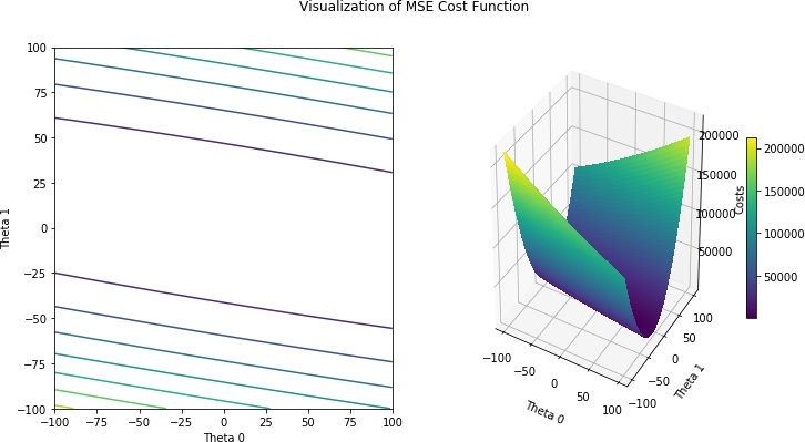
$\theta_0$ is the bias and $\theta_1$ is the slope. The next thing we need is a meassure that tells us how well a specific line fits to the data: a so called cost function $J(\theta)$. For regression we use the mean squared error:
$J(\theta) = mse(\theta) = \frac{1}{2m} \sum_{i=1}^{m} (h_{\theta}(x^{(i)} - y^{(i)})^2$,
with $m$ the number of our training examples. Squaring the distance between our prediciton $h_{\theta}(x^{(i)})$ and the true target value $y^{(i)}$ has two effects: We always get a positive value and bigger distances produce a much higher cost than smaller distances. Using the cost function we can now try different combinations of values for $\theta_0$ and $\theta_1$ and draw an error-surface, which depicts the costs depending on $\theta_0$ and $\theta_1$ and therefore how well each combination is. The following picture shows such an error-surface:
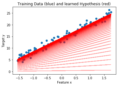
With this bruteforce method we can already solve the problem. But there is a more efficient way: gradient descent. By calculating the gradient of the cost function $\nabla J(\theta)$, which consists of the partial derivatives $\frac{\partial J(\theta)}{\partial\theta_0}$ and $\frac{\partial J(\theta)}{\partial\theta_1}$, we get to know the steepness of the cost function. Inserting concrete starting values for $\theta_0$, $\theta_1$ and our training data tells us in which diretion we have to adjust $\theta_0$ and $\theta_1$ in order to lower the costs (and to get a line that slighty fits better). Iterative calculating the gradient and updating $\theta$s, the line slowly aligns with the data:
- linear-regression slides (additional lecture notes)
- exercise-simple-linear-regression (numpy)
- exercise-pytorch-univariate-linear-regression (pytorch)
Multivariate Linear Regression
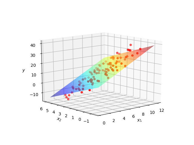
The next exercise extends the previous one, by adding more features and how to handle them the best mathematically, i.e. by making use of matrix operations and avoiding loops. By adding one more feature (having then a total of two, $x_1$ and $x_2$), we simply extend the hypothesis to $h_{\theta}(x) = \theta_0 + \theta_1 \cdot x_1 + \theta_2 \cdot x_2$. The resulting model then is no longer a straight line, but a plane:
- exercise-multivariate-linear-regression (numpy)
- exercise-pytorch-multivariate-linear-regression (pytorch)
Classification
So far we are able to build a model to predict a floating point value $y$ based on $1$ to $n$ features $x_1, \ldots, x_n$. Of course a lot of task do not require to predict a continous floating point value (e.g. temperature), but a specific class. When asked if a concrete animal is a cat or not a cat, a value in the range $]-\infty, +\infty[$ as answere does not make a lot of sense when the answere should either be a clear no (boolean $false$ or $0$) or yes (boolean $true$ or $1$). At least a normalized answere in the range $]0, 1[$, which could be interpeted as confidence / probability would be desirable.
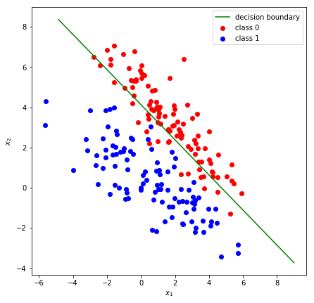
Logistic Regression
With the use of the sigmoid (or logistic) function $\sigma(z)$, the linear regression can easily be extended to predict whether a set of features of an example is likely to belong to class A or class B:
$\sigma(z) = \frac{1}{1 + exp(-z)}$,
with
$z = \theta_0 + \sum_{i=1}^m \theta_i \cdot x_i$
resulting in the new hypothesis:
$h_{\theta}(\vec x) = \frac{1}{1 + exp(- \theta_0 - \sum_{i=1}^m \theta_i \cdot x_i)}$,
The result of $\sigma(z)$ is in the range $]0, 1[$ and can be interpreted as confidence. Adding a hard threshold (e.g. at $0.5$) results in a hard binary classifier. The addition of the logistic function requires another cost function: the cross-entropy-cost:
$J(\theta) = bce(\theta) = \frac{1}{m} \sum_{i=1}^{m} (y^{(i)} \cdot ( h_{\theta}(\vec x)) + (1 - y^{(i)}) \cdot (1 - h_{\theta}(\vec x)))$
Sidenote: Although the method is called logistic regression, it is not really a regression, which only has historical reasons. In fact regression always means predicting a continous value (float), opposed to classification, where we predict a class (e.g. 0 for negative and 1 for positive).
- logistc-regression slides (additional lecture notes)
- exercise-logistic-regression (numpy)
- exercise-pytorch-logistic-regression (pytorch)
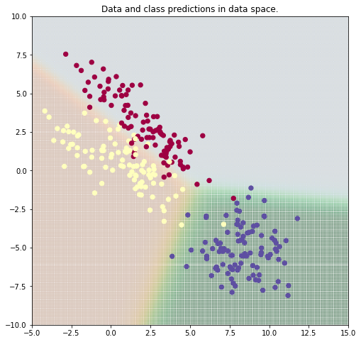
With logistic regression we are only able to differentiate between two classes. These kind of classifieres are also called binary classifiers. In order to extend the logistic regression to more than two classes, we make use of the softmax function:
$softmax(z_j) = \frac{exp(z_j)}{\sum_{k=1}^{K}exp(z_k)}$
We calculate softmax(z_j) for every class $j$ of our total number of classes $K$. The denominator in the formula is just for normalizing purpose, so we receive a value between $]0, 1[$ for every possible class, which sum up to $1.0$.
- exercise-pytorch-softmax-regression (pytorch)
Decision Trees
Of course machine learning is not only about neural networks (and therefore linear and logistic regression). There exist a lot of other algorithms, which still have their merit and justification. One example are decision trees and random forests. But before learning about the later, take a look at decision trees and the concept of entropy.
Evaluation
Until now, you have only been working with training data. But only using training data, which the model used to learn its parameters, it is hard to really tell how the model performs on unseen data. In this notebook we introduce the out-of-sample error $E_{Out}$, in contrast to the error on the training data $E_{In}$. $E_{Out}$ is composed of the variance and the bias. The ratio between these two key figures is determined by the complexity of our model and if it did not fit to the training data enough (underfitting) or even too much (overfitting). The following picture shows three models for univariate regression with varying grade of complexity:
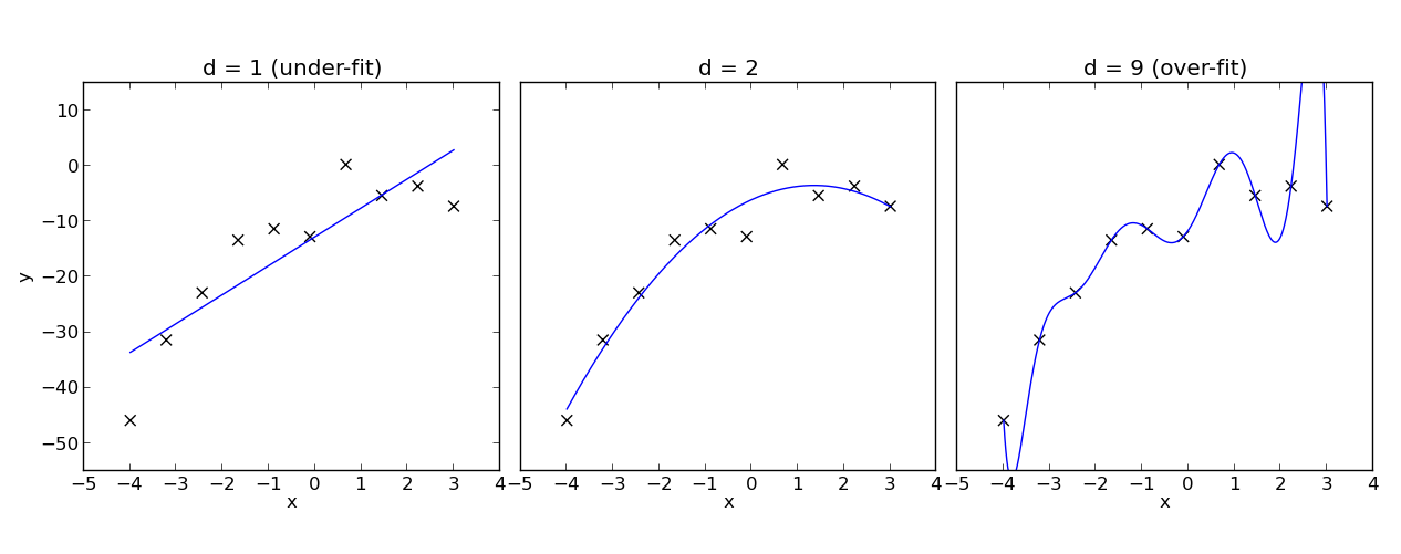
The key learning opjective in the exercise below is, that the complexity of our model is less dependant of the true target function (unknown) and more dependant on the number of available training data.
So far all the models have only been judged (good or bad) by examing the costs. In the field of machine learning, a wide variety of quality measures is beeing used. In this notebook you will get to know the most important ones, like confusion matrices, accuracy, precision and recall, f1-score and receiver-operator-characteristic.
- evaluation slides (additional lecture notes)
- exercise-evaluation-metrics
- evaluation-exercise