
Introduction
We are entering a data area. Nowadays, large data sets can be stored on commodity hardware which results in a massive decrease in storage costs. Methods for gaining value for such data become more and more critical. Machine learning promises to generate such values by learning prediction models from data. Software-libraries provide standard machine learning algorithms such a logistic regression, support vector machines and simple neural networks out-of-the-box. So they can easily be trained and used in production for simple problems.
More complicated problems require specialized models which must be designed for the problem at hand. Model-based machine learning offers a framework for modeling, learning, and inference in such models. Such models correspond to graphical representations which are called probabilistic graphical models [@Koller:2009:PGM:1795555]. For modeling, we focus on directed graphical models. In such models are Bayesian methods typically used for inference. However, Bayesian methods are a fundamental approach for data analysis and statistics. Bayesian methods have the advantage to mitigate overfitting and naturally handle uncertainty. They give a probability distribution over the predicted values. From these it can be easy concluded how confident the prediction is. Such confidence estimation is essential for critical applications, e.g., in medicine or autonomous driving.
Recently, researchers invented black-box inference for Bayesian methods. Without a black-box solver, it is necessary to implement an inference algorithm for the particular problem at hand. So in the past, only experts knew to implement such solutions. With black-box inference, machine learning developers now have the potential to develop solutions based on Bayesian methods. Based on black-box inference, probabilistic programming languages were invented to support the development process. In probabilistic programming, the developer (or researcher) can mainly focus on the modeling part by using a developer-friendly API. Still, it is essential to understand how inference works, e.g., for tuning scalable solutions or understanding the limitations.
A key trend in machine learning is deep learning. In contrast to traditional machine learning, features are learned from data and are not engineered by experts. The most prominent models are (deep) neural networks. Neural networks are typically trained with the frequentist approach, see section [sec:maximum-likelihood]. However, Bayesian methods can also be used to train neural networks or to design neural network autoencoders [sec:bayesian-deep-learning]. This paper gives the reader a guide to gain knowledge about Bayesian methods. Notably, we give pointers to exercises which we have developed for studying. We believe that seriously studying for a deep understanding cannot be done without practice. Practicing in this context is solving mathematical exercises and implementing corresponding code, e.g., algorithms. Therefore most exercises are of such a mixed type. Bayesian methods are an advanced topic of machine learning, and their study requires a strong background in machine learning. So we assume that the reader has such a background. In section [sec:fundamentals] we describe the prerequisite compactly and give links to appropriate exercises. In the next section [sec:Bayes-fundamentals], the principle of Bayesian data analysis is derived from Bayes rule, and the principal difficulty of Bayesian analysis is explained. In section [sec:Bayesian-methods] some methods are presented which overcome the difficulties. We focus on such methods which are used for probabilistic programming. In section [sec:probabilistic-programming] we describe how Bayesian inference is eased by probabilistic programming. One goal of the paper is to prepare the reader for recent research literature in the field of Bayesian (deep) learning. In section [sec:bayesian-deep-learning] we present examples of such neural networks. The complete content including the material of the exercises is equivalent to a one-semester master course for students with appropriate background in machine learning.
The exercises are based on jupyter notebooks [@Kluyver2016JupyterN]. In the exercises, we give mostly a summary of the prerequisite knowledge. Also, there are pointers to the literature for further self-study.
A complete list of all in this paper referenced exercises is given on the following web page: https://www.deep-teaching.org/courses/bayesianLearningListOfExecises
Prerequisite
Before we start with the fundamentals of Bayesian data analysis, we need some basic concepts and definitions of key technical terms. Here we assume that the reader has a fundamental background in machine learning, probability theory, and statistics.
In the following, we recapitulate some of the basics which are especially crucial for Bayesian learning.
Independent and identically distributed data
Unless otherwise stated, we assume that the data $\mathcal D = \{x_1, x_2, \dots , x_n\}$ (resp. for supervised learning $\mathcal D = \{(x_1, y_1), (x_2, y_2), \dots, (x_n, y_n)\}$ ) is independent and identically distributed ( i.i.d.):
- Independent means that the outcome of one observation $x_i$ does not effect the outcome of another observation $x_j$ for $i\neq j$.
- The data is identically distributed if all $x_i$’s are drawn from the same probability distribution.
Statistics and estimators
A statistic is a random variable $S$ that is a function of $\mathcal D$, i.e.
$S = f \left(\mathcal D \right)$
. An estimator $\hat \theta$ is a statistic used to approximate the (true) parameters $\theta$ that determine the distribution of data $\mathcal D$. The variance of an estimator is defined by
$\text{var}(\hat \theta) := \mathbb E_{\mathcal D} [\hat \theta^2] - (\mathbb E_{\mathcal D} [\hat \theta])^2.$
The subscript $\mathcal D$ on the expection $\mathbb E_{\mathcal D}$ indicates that the expectation is with respect to all possible data sets $\mathcal D$. The bias of an estimator is defined as
$\text{bias}(\hat \theta) = \mathbb E_{\mathcal D}\left[\hat \theta\right]-\theta.$
A statistic $S$ is sufficient if $p(\hat \theta \mid \mathcal D) = p\left(\hat \theta \mid S(\mathcal D)\right)$. All necessary information for the estimation of the parameters is compressed in the sufficient statistic.
For exercises, see exercise-expected-value, exercise-biased-monte-carlo-estimator, and exercise-variance-sample-size-dependence.\
Kullback-Leibler Divergence
The Kullback Leiber (KL) divergence is a measure how (dis)similar two probability distributions are. For probability mass functions $q(X)$ and $p(X)$ the KL-divergence is defined as 1: y
$\mathcal D_{KL}(q(X) \mid \mid p(X)) = \sum_{x \in \text{val}(X)} q(x) \log \frac{p(x)}{q(x)}$
$\text{val}(X)$ are the possible values of the random variable $X$. We encourage the reader to study exercise-kullback-leibler-divergence.
Directed Graphical Models
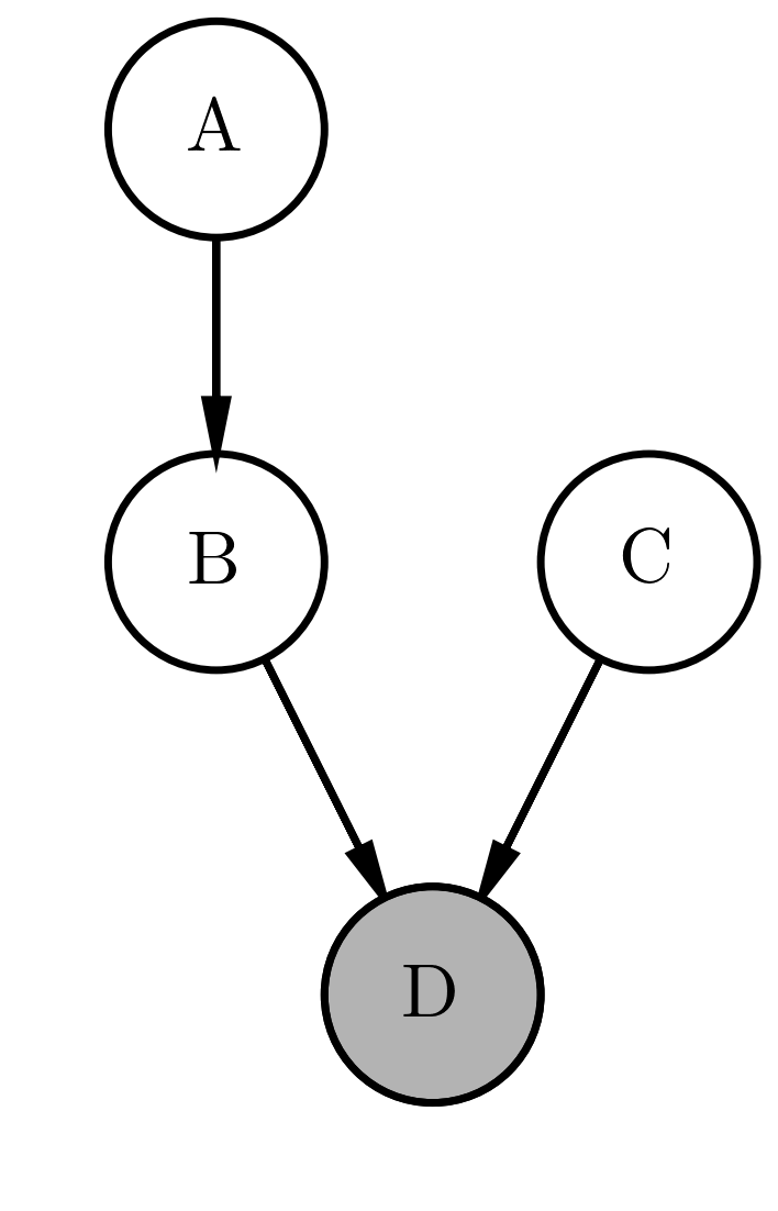
For modeling, we use the notation of directed graphical models (Bayesian networks). In a probabilistic graphical model (conditional) independence properties are encoded in the graph [@Koller:2009:PGM:1795555]. In other words a graphical model is a map of independencies (i-map). In directed graphical models, there is a set of factors corresponding to conditional probabilities for each variable. The connection between the variables is represented by a directed acyclic graphs (DAG)2. In figure [directgraphicalmodel] we give a simple example for a directed graphical model. For exercises to Bayesian networks, see
Example of a directed graphical model. A directed graphical model corresponds to a factorization of the joint probability of the random variables (nodes in the graph). Here the join probability is factorized according to $P(A,B,C,D) = P(A)P(B) P(B \mid A) P(D \mid C, B)$. If a probability factor of a random variable is conditioned on other variables an corresponding edge in the graph exists.
Fundamentals of Bayesian analysis
Bayes Rule
In the training phase the parameters of a model are learned by training data $\mathcal D$. The criteria for the learning process can be derived from Bayes rule for data $\mathcal D$ and parameters $\theta$:
$p(\theta \mid \mathcal{D}) = \frac{p(\mathcal{D} \mid \theta) p(\theta)}{p(\mathcal D)} \label{equ:bayes_rule}$
In Bayesian data analysis the continuous parameters $\theta$ of a model are described by probability density functions. Because of the importance of Bayes rule the individual factors in equation [equ:bayes_rule] have names:
- $p(\theta \mid \mathcal D)$ is called the posterior (distribution).
- $p(\mathcal{D} \mid \theta)$ is the likelihood. Typically, the likelihood is considered as a function of $\theta$, i.e. $\ell(\theta) = p(\mathcal{D} \mid \theta)$. Note that $\ell(\theta)$ is not a probability distribution with respect to $\theta$.
- $p(\theta)$ is the prior. This distribution describes the prior knowledge (or belief) about $\theta$ before taking the data $\mathcal D$ into consideration.
- The denominator on the right side $p(\mathcal D)$ is the marginal likelihood or evidence. In practice, the denominator $p(\mathcal D)= \int_\Theta p(\mathcal D \mid \theta) p(\theta) d \theta$ is often computationally untractable. Different methods were developed to handle this issue, see section [sec:Bayesian-methods].
We provide an exercise for studying Bayes rule exercise-bayes-rule.
Prediction
To predict new data $\mathcal{\bar D}$ 3 based on the training data $\mathcal D$ we have to average the preditions $p(\mathcal{\bar D} \mid \theta)$ weighted by the posterior $p(\theta \mid \mathcal{D})$
$\begin{aligned} p(\mathcal{\bar D} \mid \mathcal{D}) &= \int_\Theta p(\mathcal{\bar D}, \theta \mid \mathcal D) d\theta \\ &= \int_\Theta p(\mathcal{\bar D} \mid \theta, \mathcal D) p(\theta \mid \mathcal{D}) d\theta \label{aa}\\ &= \int_\Theta p(\mathcal{\bar D} \mid \theta) p(\theta \mid \mathcal{D}) d\theta \label{bb}\end{aligned}$
$\Theta = \{\theta \mid P(\theta \mid \mathcal{D}) >0\}$ is the support of $P(\theta \mid \mathcal{D})$. From line [aa] to [bb] the conditional independence property $\mathcal{\bar D} \perp \mathcal{D} \mid \theta$ was used.
Maximum Likelihood Estimation (ML)
In comparision to Bayesian data analysis in a frequentist approach the parameters $\theta$ are estimated by fixed values (point estimates), i.e. they are not described by probability distributions. Typically $\theta$ is estimated by maximizing the likelihood $\ell(\theta)$, i.e. by $\hat \theta_{ML} = \arg\max_\theta \ell(\theta)$. This is equivalent to minimizing the negativ log-likelihood $\log \ell(\theta) = L(\theta)$
$\label{equ:ML-estimation} \hat \theta_{ML} = \arg\max_\theta \ell(\theta) = \arg\min_\theta \left(- \mathcal \log \left( \ell(\theta) \right) \right) = \arg\min_\theta \left(- L (\theta) \right)$
As simple example we consider the Binomial distribution. From $n$ identical Bernoulli trials with possible outcomes $x_i = \{0,1\}$ we get some data, e.g. $\mathcal D=\{0,1,1,\dots\}$. From the data we want to estimate the parameter $\theta$. Here $\theta$ is the probability of a positive outcome $X = 1$ of a Bernoulli trial.\ From the data we can compute a sufficient statistics which holds the same information about $\theta$ as $\mathcal D$. The suffient statistics for the Bernoulli distribution is the number of sucesses ($1$’s) $k$ and the number of trials $n$. The probability for $k$-sucesses is given by
$\label{equ:binominal_distribution} P( k \mid \theta) = {n \choose k} \theta^k (1-\theta)^{n-k}$
If we consider this as a function of $\theta$ we get the likelihood. For the maximum-likelihood estimation for the Binomial distribution we have:
$\arg\min_\theta \left( - \mathcal \log L(\theta) \right)= \arg\min_\theta - \log \left( {n \choose k} \theta^k (1-\theta)^{n-k}\right)$
A necessary condition for the minimum is that the first derivative is zero:
$0 = \frac{d}{d\theta} \left( \theta^k (1-\theta)^{n-k}\right) = k \theta^{k-1} (1-\theta)^{n-k} - (n-k) \theta^{k} (1-\theta)^{n-k-1}$
So the maximum likelihood estimator is $\hat \theta_{ML} = \frac{k}{n}$. For an exercise to maximum-likelihood on the Gaussian distribution see exercise-univariate-gaussian-likelihood.
Another point estimate is given by the maximization of the posterior of equation [equ:bayes_rule] ( maximum a posterior - MAP). Note that the denominator is constant with respect to (w.r.t.) $\theta$. Therefore for maximization, it is sufficent to consider only the prior and the likelihood. In log-space the prior and the likelihood are added. E.g., for learning a linear regression (or neural networks regression) the Squared error loss correspond to the log-likelihood and the L2-regularization term to a Gaussian log-prior. We provide exercise-linear-regression-MAP for studying the derivation in detail.
Hidden variable models, expectation maximization and variational lower bound
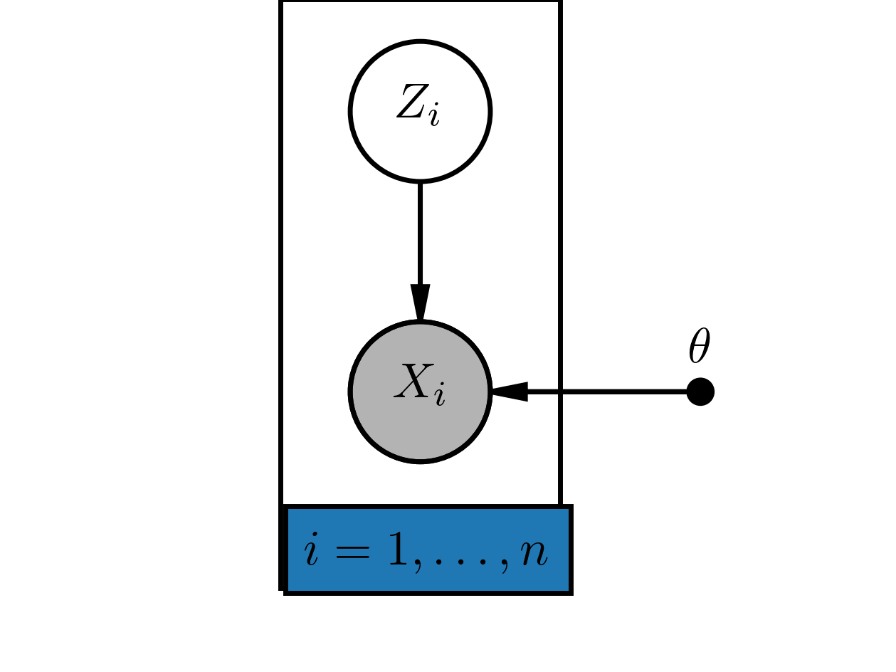
Bayesian networks can contain unobserved variables. Sometimes we are interested in the distribution of such variables when we observe other variables in the graph. As example consider a mixture of two Gaussians 4 with indices $z=1$ respectivly $z=2$. Each of the Gaussians has two parameter $(\mu_z, \sigma^2_z)$ with $z \in \{1,2\}$. Given some i.i.d. training data $\mathcal D = \{x_1, \dots, x_n \}$ we want to estimate the parameters $\theta = \{\mu_1, \sigma_1^2, \mu_2, \sigma_2^2\}$ by maximum likelihood. Additionally, we want to know for each (training) example the distribution $p(z_i \mid x_i)$.\ To summerize the problem we have a set of hidden variables $z_i$. Here we have for each hidden variable an observation $x_i$. In figure [HVM-model] there is a graphical representation of this hidden variable model.
Example of a simple hidden variable model: For each observed variable $X_i = x_i$ there is a hidden variable $Z_i$.
For the training data we want a point estimate of $\theta$ and a probability distribtion $p(z_i \mid x_i; \theta)$. So we are Bayesian only w.r.t. $z_i$.\ The (marginal) 5 log-likelihood of the observed data is:
$\label{equ:hvm-log-likelihood} L(\theta) = \log p({\mathcal D} \mid \theta) = \sum_{i}^n \log p({x}_i \mid \theta ) = \sum_{i=1}^n \left(\log \sum_{z_i} p(x_i, z_i \mid \theta )\right)$
The difficulty is that we don’t know from which Gaussian $z$ each data point was generated. This is reflexted in the formula [equ:hvm-log-likelihood]. There is a sum inside the $\log$ which complicates the maximization procedure substantially.\ However, with the Jensen inequality and an auxilary distribution $q(z_i)$ we can push the $\log$ inside the sum to get a lower bound [@Neal:1999]:
$\begin{aligned} \label{equ:lower-bound} L(\theta) &= \sum_{i} \log p(x_i \mid \theta ) \\ & = \sum_{i=1} \left(\log \sum_{z_i} p(x_i, z_i \mid \theta )\right) \\ & \geq \sum_{i} \sum_{z_i} q(z_i) \log \frac{p(x_i, z_i \mid \theta )}{q(z_i)} \\ & = \sum_{i} \mathbb E_{q(z_i)} \left[\log \frac{p( x_i, z_i \mid \theta )}{q(z_i)}\right] \\ & = - \sum_{i} \mathcal D_{KL} \left( q(z_i) \mid \mid p(x_i, z_i \mid \theta ) \right) \label{equ:lower-bound_1}\\ & = \mathcal L(q, \theta)\end{aligned}$
$\mathcal L(q, \theta)$ is the variational lower bound (or evidence lower bound - ELBO). Note that $\mathcal L(q, \theta)$ has two arguments $q$ and $\theta$. Iteratively alternating until convergence between the maximization of one holding the other argument fixed results in the EM-algorithm, with interation index $t$:
- In the E-Step we search in the distribution family $q$ at the current position $\theta^{(t)}$ the strongest bound: $q^{(t+1)} \leftarrow \text{arg} \max_q \mathcal L(q,\theta^{(t)})$
- In the M-Step we maximize for a fixed $q^{(t+1)}$) w.r.t. $\theta$: $\theta^{(t+1)} \leftarrow \text{arg} \max_{\theta} \mathcal L(q^{(t+1)},\theta)$
The gap between the lower bound $\mathcal L (q, \theta)$ and the log-likelihood $L(\theta)$ is6:
$\begin{aligned} L(\theta) - \mathcal L (q, \theta) = \sum_{_i} \mathcal D_{KL}\left( q({\bf z}_i) \mid \mid p({\bf z}_i \mid {\bf x_i}, \theta )\right )\end{aligned}$
We provide two exercises to study the EM algorithm in detail:
- Minimalistic example of a hidden variable model which should be solved by the EM-algorithm: exercise-simple-example-for-EM
- One dimensional Gaussian mixture model trained with the EM-Algorithm: exercise-1d-gmm-em
Remark: If we want to estimate a probability distribution of the parameters $\theta$, i.e. $p(\theta \mid \mathcal D)$ we can consider the parameter as hidden variables. So the distinction between parameters and variables is blurred in Bayesian analysis.
Bayesian Methods
Different Bayesian methods were developed to compute respectivly approximate the posterior of equation [equ:bayes_rule] without explicitly computing the denominator. Here we focus on Monte Carlo methods and variational methods for which black-box inferences were developed recently. For didactic reasons, we also explain the conjugate prior method to illustrate the principle of Bayesian learning.
Conjugate Prior
For simple models, the conjugate prior method can be used to overcome the problem for computing the denominator of equation [equ:bayes_rule]: For the prior $p(\theta)$ and the likelihood $p(\mathcal D \mid \theta)$ are such probability functions selected such that the posterior has the same functional form as the prior (same family of functions). To illustrate this, we consider again $n$ Bernoulli trials. So for the likelihood we have the Binominal distribution, see equation [equ:binominal_distribution]. If we use for the prior probability density function (pdf) the Beta distribution then the posterior is again a Beta distribution.\ The Beta distribution is
$\begin{aligned} \text{Beta}(\alpha, \beta) = p(\theta \mid \alpha,\beta) & = \frac{\theta^{\alpha-1}(1-\theta)^{\beta-1}}{\int_0^1 u^{\alpha-1} (1-u)^{\beta-1}\, du} \label{equ:beta_distribution}\end{aligned}$
with $\theta \in { } [0,1]$ and the shape parameters $\alpha > 0, \beta > 0$. Note that the denominator only normalizes the pdf. Now we neglect all normalizing constants to compute the (unnormalized) posterior. The product of the (unnormalized) prior and the (unnormalized) likelihood is
$p(\theta \mid n, k ) \propto \theta^k (1-\theta)^{n-k} \theta^{\alpha-1}(1-\theta)^{\beta-1} = \theta^{k+\alpha-1}(1-\theta)^{n-k+\beta-1} \label{equ:beta_binominal}$
Comparing the right side of equation [equ:beta_binominal] with the nominator of equation [equ:beta_distribution] we see that the functional form is identical. Therefore we can conclude that the posterior is also a Beta distribution $\text{Beta}(\alpha', \beta')$ with parameters $\alpha' = \alpha + k$ and $\beta' = \beta + n - k$.
The conjugate prior method is used, e.g. for sensor fusion and in the Kalman Filter7 (to combine the measurement with the motion dynamics/kinematics). We provide an exercise for sensor fusion and Kalman Filter: exercise-sensorfusion-and-kalman-filter-1d.
As already stated, the conjugate prior method can only applied to simple problems with standard probability density functions. To allow arbirary probability densities we need more flexible methods. The first one we consider are Monte Carlo methods.
Monte Carlo Methods
Monte Carlo (MC) methods are a general approach to get approximations for numerical results. For example, Monte Carlo methods can be used to approximate integrals (Monte Carlo integration). Here we consider integrals witch contain a factor $p(x)$ in the integrand, as for computing expectations or marginalization. If we can draw $m$ samples $x_i$ from a probability distribution $p(x)$ (notated as $x_i \sim p(x)$) we can get an approximation by the crude MC estimator
$F(x) = \int p(x) f(x) dx \approx \sum_{i=1}^m f(x_i) = \hat F(x). \label{equ:crude_mc_estimate}$
See also exercise-sampling-crude-monte-carlo-estimator.\ But how to obtain samples from $p(x)$? If $x$ is a scalar and we know the cumulative distribution function (cdf) $c(x) = \int_{-\infty}^x p(x') dx'$ we can sample by inverse transform sampling: First we draw samples from a uniform distribution $\text{uniform}(0,1)$ by a random number generator. Then these samples are maped by the inverse cdf, see exercise exercise-sampling-inverse-transform..
For different standard multivariate probability distributions there are several methods for sampling, see e.g. [@numerical_recipies chapter 7]. Many software packages (e.g. numpy.random) implement such sampling for standard probability distributions out-of-the-box. Such sampling methods can also be used for other applications. We provide exercises for the following sampling methods:
- In rejection sampling the samples are drawn from a similar probability distribution $q(x)$. Some of the samples are rejected to get samples from $p(x)$ as result, see exercise-sampling-rejection.
- In importance sampling the samples are also drawn from similar distribution $q(x)$. These samples are weighted by the ratio $p(x)/q(x)$, e.g. to correct the Monte Carlo integration, see exercise
https://www.deep-teaching.org/notebooks/monte-carlo-simulation/sampling/exercise-sampling-importance[exercises-sampling-importance]{}.
Gradient of a MC expectation
Often the gradient of an expectation is needed, e.g. for optimization by gradient descent, see section [sec:bayesian-deep-learning] for examples. By algebraic manipulation the gradient of an expectation can be expressed by the expectation of a gradient:
$\nabla_w \mathbb E_{q_w(x)} \left[f(x)\right] = \mathbb E_{q_w(x)} \left[f(x)\nabla_w \log q_w(x) \right]$
The expectation on the right hand side can be approximated by Monte Carlo if we can sample from $x_i \sim q_w(x)$. That is the so-called score function estimator trick.
TODO exercise!!
Variance reduction
Monte Carlo methods give an estimate and not an exact solution. The estimated value should be as close as possible to the true value. So the estimate should have low variance and should be unbiased. There are different methods to reduce the variance of an MC-estimator. Often, only by such variance reduction, Monte-Carlo becomes practical. For some of the variance reduction techniques we provide exercises:
- Control Variates 8: exercise-variance-reduction-by-control-variates
- Reparametrization: exercise-variance-reduction-by-reparametrization
- Rao-Blackwellization: exercise-variance-reduction-by-rao-blackwellization
Markov Chain Monte Carlo (MCMC)
In principle, the normalized posterior of equation [equ:bayes_rule] can be approximated with Monte Carlo integration by an MC-estimate of $p(\mathcal D)=\int p(\theta) p(\mathcal D\mid \theta) d\theta$. The variance of such an estimator would be very high except $\theta$ is very low dimensional. So this method can not be used in practice.\ Note that if the probability space is high dimensional $\theta$ then in most regions is $p(\theta)\approx0$. If we would for example use importance sampling, e.g. by direct sample from a uniform distribution and weighting then most importance weights would be zero. So the effective number of samples would be extremly low. This results in a very high variance of the estimator.\ Therefore we want to draw only samples from regions where $p(\theta)$ is substantially different from zero. If we have such a sample $\theta^{(t)}$ at iteration step $t$ then is highly probable that nearby values of $\theta^{(t)}$ have also $p(.)$ substantially different from zero. The idea of MCMC is now to perturbe the current sample $\theta^{(t)}$ by a small $\delta \theta^{(t)}$. Such, we get a candidate $\theta_c{(t+1)}=\theta^{(t)}+\delta \theta^{(t)}$. We accept the move only with an acceptance probability $p_{ac}$ \cite{} given by
$p_{ac}= \min\left(1, \frac{ p\left(\theta^{(t)}\right) p \left( \theta_c^{(t+1)} \mid \theta^{(t)} \right)} { p\left(\theta_c^{(t+1)}\right) p \left( \theta^{(t)} \mid \theta_c^{(t+1)} \right)} \right),$
i.e. with $p_{ac}$ we accept the move and with $1-p_{ac}$ we stay at the value $\theta^{(t)}$:
$\theta^{(t+1)} = \begin{cases} \theta_c^{(t+1)} & \text{with probability } p_{ac} \\ \theta^{(t)} & \text{with probability } 1-p_{ac} \end{cases}$
The new state $\theta$ at $t+1$ depends only on the previous state at $t$ and is independent of the states previous to $t-1$. Therefore the Markov property $\theta^{(t+1)} \perp \theta^{(t-1)} \mid x^{(t)}$ is satisfied and such a sampling is called Markov Chain Monte Carlo. State-of-the-art of MCMC is the Nuts sampler [@NUTS] which is an improvement of Hamiltonian MCMC [@hamiltonian_mcmc].
TODO: exercise-sampling-direct-and-simple-MCMC.ipynb
Variational Methods
A drawback of MCMC is that it is not scalable to large data sets or models with many parameters. For such models, MCMC is typically very slow, and we need many samples. Therefore, it can not be used in practice. Alternatives are variational methods to overcome these issues.
The idea of variational methods is to approximate $p(\theta \mid \mathcal D)$ with a so-called variational distribution $q_w(\theta)$. $q_w(\theta)$ is a distribution in a parametrized family, i.e., we chose a standard probability distribution with parameters $w$s. The parameters $w$ are called variational parameters. Then, we must find the $w$’s which approximate the posterior best by an optimization procedure like stochastic gradient descent.\ As optimization-objective (loss) we use the KL-Divergence between $q_w(\theta)$ and $p(\theta \mid \mathcal D)$, i.e. the optimal parameters are $w^* = \text{arg} \min_w \mathcal D_{KL} \left(q_w(\theta)\mid\mid p(\theta \mid \mathcal D) \right)$.
$\begin{aligned} \mathcal D_{KL} \left( q_w(\theta) \mid \mid p( \theta \mid \mathcal D ) \right) &= \int_\Theta q_w(\theta) \log \frac{q_w(\theta)}{p(\mathcal D \mid \theta)p(\theta)} d \theta + \int_\Theta q_w(\theta) \log p(\mathcal D ) d \theta \\ &= \int_\Theta q_w(\theta) \log \frac{q_w(\theta)}{p(\theta)} d \theta - \int_\Theta q_w(\theta) \log p(\mathcal D \mid \theta) d \theta + \log p(\mathcal D ) \\ &= \mathcal D_{KL} \left( q_w(\theta) \mid \mid p(\theta) \right) - \mathbb E_{q_w(\theta)} \left[ \log p(\mathcal D \mid \theta) \right] + const.\end{aligned}$
Note that $\log p(\mathcal D )$ does not depend on $w$ which prevents us from the difficulty to compute the “normalizer” of the posterior (denominator of equation [equ:bayes_rule]). $q_{w^*}(\theta)$ is an approximation of $p(\theta \mid \mathcal D)$. Remember that we are using a known parametric distribution for $q_w(\theta)$, so we have a normalized result.
Mean-field approximation
For a directed graphical model with many nodes, the probability distribution for each node $j$ is described by a known parametric distribution $q_w(\theta_j)$ and the total probability distributions factorizes9:
$Q = \left\{ q_w \mid q_w(\theta)= \prod_j q_{w^{(j)}}(\theta_j)\right\}$
This factorization approach is called mean-field approximation. The optimization can be done by coordinate descent, i.e. by a loop over the optimation w.r.t. to each $q_{w^{(j)}}(\theta_j)$ until convergence.
We provide the following exercises for studying:
- exercise-variational-mean-field-approximation-for-a-simple-gaussian - univariate Gaussian via variational mean field.
- exercise-variational-EM-bayesian-linear-regression Bayesian univariate linear regression model via mean field approximation and variational expectation maximization (for the data noise a point estimate should be used).
Probabilistic programming
Probabilistic programming allows defining models similar to (directed) graphical models programmatically. The modeling in probabilistic programming is more powerful because the model can contain control structures such as loops and if-statements. It can be show, that every directed graphical model can be expressed by a loop-free probabilistic program [@Gordonprobabilisticprogramming].\ Inference (including learning) is based on black-box methods based on MC sampling or variational inference @automatedVI; @blackbox_VI. Therefore, the programmer can focus primarily on modeling. Depending on the software packages the inference is entirely automatic, or it requires strong background knowledge for tuning the inference. Such tuning is especially necessary for a large data set and big models.
The source code for a simple Gaussian model with pyro [@bingham2018pyro] and the corresponding variational distribution model is show in figure [fig:pyro_gaussian].
def model(X): mu = pyro.sample(’mu’, dist.Uniform(-10., 10.)) return pyro.sample(’gaussian_data’, dist.Normal(mu, 1.), obs=X)
def guide(X): mu_loc = pyro.param(’guide_mu_mean’, torch.randn((1))) mu_scale = pyro.param(’guide_mu_scale’, torch.ones(1), constraint=constraints.positive) pyro.sample(’mu’, dist.Normal(mu_loc, mu_scale))
We provide the following exercises for probabilistic programming:
Bayesian Deep Learning
In this section, we give two non-trivial examples from deep learning for which we provide exercises. In both examples, the neural networks are trained by variational methods lower. Nevertheless, Monte-Carlo estimation is used for approximate the gradient of the expectations of the lower bound.
Variational Autoencoder
Variational Autoencoders [@autoencodedvariational_bayes] are generative models which can learn complicated probability distributions. Variational autoencoder are hidden variable models. So the terminology and the graphical model 11 are analog to section [sec:hidden-variable-models]. The variational autoencoder is trained by the auto-encoding variational bayes (AEVB) algorithm. In contrast to the EM-algorithm can AEVB be used if the integral of the marginal likelihood $\int p(Z\mid \theta)p(X=x_i \mid Z; \theta) dZ$ is intractable [@autoencodedvariational_bayes]. An other advantage is, that AEVB can be trained by minibatches for large data sets. $q_w(Z \mid x_i)$ is the variational approximation of $p(Z \mid x_i; \theta)$. Note that the approximation depends explicitly on $x_i$ 12. $q_w(Z \mid x_i)$ is implemented by an probabilistic encoder neural network 13. The weights and biases of the encoder neual network are the variational parameters $w$. In the training phase the probabilistic encoder maps each input $x_i$ to a probabilistic (variational) approximation $q_w(Z \mid x_i)$ of the true posterior $p(Z \mid x_i; \theta)$. In deep learning terminology the hidden state distribution $p(Z \mid x_i; \theta)$ is a probabilistic representation of the input $x_i$. $x_i$ is encoded “truely” by $p(Z \mid x_i, \theta)$ approximated by $q_w(Z \mid x_i)$.
Additionally, there is a second neural network that acts as a probabilistic decoder. The task of the decoder is to reconstruct the input $x_i$ from a sample $z_i \sim q_w(Z \mid x_i)$, i.e. the decoder implements $p(x_i \mid Z; \theta)$\ For training, the (negative) evidence lower bound as cost function used 14:
$\label{elbo-VAE} \mathcal L(w, Z) = \sum_i \left( \mathbb E_{q_w(Z\mid x_i)}[\log p(x_i \mid Z; \theta)] - D_{KL}[q_w(Z \mid x_i) \mid \mid p(Z)] \right)$
The first term on the right hand side is a measure of the reconstruction error. The second term acts as a constraint (regularization), the representations of the training data should be similar to samples from a prior. As prior we chose typically a centered isotropic multivariate Gaussian. That is a Gaussian with zero mean-vector and diagonal covariance matrix $\mathcal N (0, \mathbb 1)$ with entries $1$. For optimization w.r.t. the variational parameters $w$ we must compute the gradient of equation [elbo-VAE]. The second term can be integrated analytically for a Gaussian prior and Gaussian conditionals $p(x_i \mid Z;\theta)$ [@autoencodedvariational_bayes]. The closed form allows directly automatic differentiation for optimization.\ The gradient of the first term can be approximated by Monte Carlo estimation, see section [sec:gradient-mc]. However, the score function estimator has to high variance and can therefore not be used. This is solved by the reparametrization technique for variance reduction (see section [sec:variance_reduction]) . With reparametrization we can also backprop through the encoder decoder network. For details see [@autoencodedvariational_bayes] and our exercise exercise-variational-autoencoder
A learned auto-encoder can generate as many samples as wanted. First, a sample is drawn from the prior $p(Z)$, i.e., the multivariate Gaussian with diagonal covariance matrix $\mathcal N (0, \mathbb 1)$. The decoder then maps the Gaussian sample to a sample from the learned distribution.
Bayesian Neural Networks
Neural networks are typically learned by minimizing a cost function, e.g., the cross-entropy loss with additional regularization. This is equivalent to a MAP point estimate, see section [sec:maximum-likelihood].\ In Bayesian Neural Networks the weights are represented by probability density functions [@Hinton:1993]. Typically the mean-field approximation (see section [sec:mean-field]) is used for Bayesian Neural networks. The complete probability distribution factorizes such that each weight corresponds to a univariate Gaussian 15. Each weight $\theta_j$ has two (variational) parameters $w_j$ the mean and the variance of the Gaussian $w_j=\{mu_j, \sigma_j^2\}$, i.e. $p(\theta) \approx \prod_j q_{w_j}(\theta_j)$ with Gaussians $q_{w_j}(\theta_j) = \mathcal N(\mu_j, \sigma_j^2)$. Such networks can be trained by backprop for learning of the variational parameters $w_j$. As cost the lower bound (analog to equation [elbo-VAE]) can be used. For details see [@bayesbybackprop] and our exercise exercise-bayesian-by-backprop.
Conclusion and Outlook
In the paper we gave an guide to learn Bayesian methods with a focus on machine and deep learning. Mainly, we provide a set of different exercises for studying the material in detail. In the future, we want to review, improve and extend the exercises and provide more exercises related to Bayesian learning and the corresponding fundaments.
Most of the exercises were developed in the project Deep.Teaching. The project Deep.Teaching is funded by the BMBF, project number 01IS17056.
-
For probability density functions the sum must be replaced by an integral.
↩ -
For a short summary (in German) of Bayesian networks, see http://christianherta.de/lehre/dataScience/bayesiannetworks/BayesscheNetze_Repraesentation.html
↩ -
An analog expression for supervised learning $p(\bar y \mid \mathcal D, \bar x)=\int p(\bar y\mid \bar x; \theta) p(\theta \mid \mathcal D) d\theta$ can be derived from the conditional independencies.
↩ -
For an exercise to the multivariate Gaussian distribution see exercise-multivariate-gaussian
↩ -
The marginalization is with respect to hidden variables $z_i$
↩ - ↩
-
For an derivation of the Kalman Filter in the simple 1d case see e.g. http://christianherta.de/lehre/localization/Kalman-Filter-1D.html
↩ -
In the context of reinforcement learning this is known as baseline.
↩ -
In general the probability can factorizes in blocks, e.g. a block for each node, or total factorization for each component $\theta_i$. This can be expressed by merging or spitting of nodes in the graphical model.
↩ -
Variational methods, as well as the Nuts/Hamiltonian-MC sampler, need gradient information, therefore, is probabilistic programming often implemented on top of deep learning libraries which support (reverse) automatic differentiation [@automatic_differentiation].
↩ -
There is also an arrow from $\theta$ to $Z_i$.
↩ -
So we need only a global set of variational parameters which can be used for each data point $i$. In the literature this is also called amortization.
↩ -
Note that the mean-field approximation is not used and the approximation is therefore not necessarily factorial.
↩ -
The reader is strongly encourage to compare this with formula [equ:lower-bound_1] and to derive the equivalence.
↩ -
Note that this is equivalent to a multivariate Gaussian distribution with diagonal covariance matrix for all weights.
↩